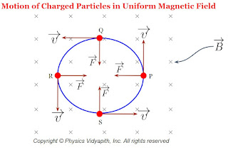
Motion of Charged Particles in Uniform Magnetic Field

Description:

The motion of any particle is depends upon the force applying on it. In the magnetic field, the motion of charge is perpendicular to the magnetic force applied on the charge particle because of that the path of the charge particle becomes circular. If the direction of force and the direction of motion are not perpendicular to each other that is they are at any angle then the path of the charge particle becomes becomes helical.

A.) When $\overrightarrow{v}$ is perpendicular to $\overrightarrow{B}$→

Let us consider a charge $q$ enters in the magnetic field $\overrightarrow{B}$ from a point $O$ with velocity $\overrightarrow{v}$ directed perpendicular to the magnetic field $\overrightarrow{B}$.The general Expression for the force acting on the particle is

$\overrightarrow{F}=q(\overrightarrow{v} \times \overrightarrow{B})$

Here the magnetic field $\overrightarrow{B}$ is perpendicular to the plane of the page directed downwards which is shown in the figure below.

Since the velocity of charge particle $\overrightarrow{v}$ is perpendicular to the magnetic field $\overrightarrow{B}$ then the magnitude of the force $F$ will be

$F=qvB \qquad(1)$

Since the force is perpendicular to the velocity and the direction of velocity continuously changes but the magnitude of velocity is not changing. Therefore the particle will move in a circular path with constant speed in a uniform magnetic field and the magnetic force will act as a centripetal force. i.e.

$F=\frac{m v^{2}}{r} \qquad(2)$

Where
$r$ → Radius of the circular path
$m$ → mass of the particle

From equation $(1)$ and equation $(2)$

$\frac{m v^{2}}{r}=qvB$

$r=\frac{mv}{qB}$

The direction of the path of the particle depends upon the nature of the charge and the direction of the magnetic field.

The particle travels a distance $2\pi r$ in one revolution. So the time period of one revolution is

$T=\frac{2\pi r}{v} \qquad(3)$

Now substitute the value of $r=\frac{mv}{qB}$ in equation $(3)$ then we get

$T=\frac{2\pi m}{qB}$

The frequency of the particle $n=\frac{1}{T}$ can be written as

$n=\frac{qB}{2\pi m}$

From the above equations, We can conclude that the time period or frequency of the particle is independent of the speed $v$ of the particle. If the speed of the charge particle increases, its radius also increases so that the time taken to complete one cycle or revolution remains the same. If two identical charged particles enter the field with different speeds $v_{1}$ and $v_{2}$, then they move along the circle of smaller and larger radii respectively which is shown in the figure below.

The frequency and Time period of the particle are independent of the speed

B.) When $\overrightarrow{v}$ is not perpendicular to $\overrightarrow{B}$→

Now, Again Let that the particle is entering with velocity $\overrightarrow{v}$ in the magnetic field $\overrightarrow{B}$, instead of being perpendicular to $\overrightarrow{B}$, makes angle $\theta (0 < \theta < 90^{\circ})$ with it. Now the velocity $\overrightarrow{v}$ may resolved into two components;

First is:

$v_{\parallel}=v \: cos\theta$ i.e. Parallel to magnetic field $\overrightarrow{B}$. This component gives the linear path to the particle.

Second is:

$v_{\perp}=v \: sin\theta$ i.e. Perpendicular to magnetic field $\overrightarrow{B}$. This component gives the circular path to the particle.

The resultant of these two-component gives the helical path to the particle whose axis is parallel to the magnetic field.

The radius of the circular path of the helix is

$r=\frac{mv_{\perp}}{qB}$

$r=\frac{mv \: sin\theta}{qB}$

Helical Motion of Charged Particle

The time period of the particle

$T=\frac{2\pi m}{qB}$

The linear distance traveled by the particle in the direction of the magnetic field in one complete circle is called the 'pitch $(p)$' of the path.

$p=v_{\parallel} \times T$

$T= v \: cos\theta \times \frac{2\pi m}{qB}$

Kinetic Energy of Charged Particle Moving in Uniform Magnetic Field→

The kinetic energy is

$K=\frac{1}{2}mv^{2}$

$K=\frac{(mv)^{2}}{2m}$

Now substitute the value of $mv$ from $r=\frac{mv}{qB}$. Then we get

$K=\frac{1}{2}m \left( \frac{rqB}{m} \right)^{2}$

$K=\frac{r^{2}q^{2}B^{2}}{2m}$

Read More

Normalized and Orthogonal wave function

Description:

We know that $\psi^{*}\psi$ or $\left|\psi \right|^{2} d\tau $ represent the probability of finding the particle in volume element $d\tau$.

The total probability of finding the particle in the entire space is 1 so

$ \int \left|\psi(r,t) \right|^{2} d\tau=1 $

Where integral extends overall space.

$\int \psi^{*}(r,t) \psi(r,t) d\tau=1$

A wave function satisfies the above equation so it is called normalized to unity. For any wave function that is a solution of the time-dependent Schrodinger equation

$\int \psi^{*} \psi d\tau=N$

$\frac{1}{N} \int \psi^{*} \psi d\tau=1$

$\int \frac{\psi{*}}{\sqrt{N}} \frac{\psi}{\sqrt{N}} d\tau = 1$

Where
$\sqrt{N}$ → Normalized Factor
$\frac{\psi}{N} $ → Normalised wave function

If independent coordinate $x$,$y$,$z$, and $\psi$ satisfy the Schrodinger wave equation. Then it is evident that $\frac{\psi}{\sqrt {N}}$ also satisfies the Schrodinger wave equation.

If $\psi_{i}$ and $\psi_{j}$ are two different wave functions both the satisfactory solution of the wave equation for a given system. Then these functions will be normalized if

$\psi_{i}^{*} \psi_{i} d\tau=1 \quad and \quad \psi_{j}^{*} \psi_{j} d\tau=1$

If the two wave function $\psi_{i}$ and $\psi_{j}$ are the satisfactory solution of the wave equation for a given system. Then these functions will be mutually orthogonal if

$\psi_{i}^{*} \psi_{j} d\tau=0 \qquad Where \: $i \neq j$

$\psi_{j}^{*} \psi_{i} d\tau=0 \qquad Where \: $i \neq j$

These integral vanishes over the entire space.

Read More

Quantum Mechanical Operators

Operator →

An operator is defined as a mathematical term that is used in the operation of a function so that this function may or may not be transformed into another function.

Operators of Quantum Mechanics →

There are the following quantum mechanical operators which are used in the wave function of particles:-

Momentum Operator

Kinetic Energy Operator

Total Energy Operator (Hamiltonian Operator)

Total Energy Operator in terms of the differential with respect to time

Momentum Operator →

The wave function for a free particle moving along the position $x$-direction is

$\psi(x,t)=A e^{\frac{i}{\hbar}(P_{x}x-Et)}$

Differentiate the above equation with respect to $x$ then we get

$\frac{\partial \psi}{\partial x}= A e^{\frac{i}{\hbar}(P_{x}x-Et)} \frac{i}{\hbar} P_{x} $

$\frac{\partial \psi}{\partial x}= \psi \frac{i}{\hbar} P_{x} $

$ P_{x} \psi = \frac{\hbar}{i}\frac{\partial \psi}{\partial x}$

$ P_{x} = \frac{\hbar}{i}\frac{\partial}{\partial x}$

For three dimensional:-

$\overrightarrow{P}= \frac{\hbar}{i} \overrightarrow{\nabla}$

Kinetic Energy Operator →

We know that the momentum operator

$ P_{x} \psi = \frac{\hbar}{i}\frac{\partial \psi}{\partial x} \qquad(1)$

Differentiate the above equation $(1)$ with respect to $x$ then we get

$ P_{x} \frac{\partial \psi}{\partial x} = \frac{\hbar}{i}\frac{\partial^{2} \psi}{\partial x^{2}} \qquad(2)$

Now substitute the value of $\frac{\partial \psi}{\partial x}$ from equation $(1)$ to equation $(2)$

$\frac{\hbar}{i}\frac{\partial^{2} \psi}{\partial x^{2}} = P_{x} \frac{i}{\hbar} P_{x} \psi$

$\frac{\hbar^{2}}{i^{2}}\frac{\partial^{2} \psi}{\partial x^{2}} = P_{x}^{2} \psi$

$ -\hbar^{2}\frac{\partial^{2} \psi}{\partial x^{2}} = P_{x}^{2} \psi \qquad (\because i^{2}=-1)$

$ -\frac{\hbar^{2}}{2m}\frac{\partial^{2} \psi}{\partial x^{2}} = \frac{P_{x}^{2}}{2m} \psi \qquad {3}$

$ -\frac{\hbar^{2}}{2m}\frac{\partial^{2} \psi}{\partial x^{2}} = K \psi \qquad (\because \frac{P_{x}^{2}}{2m} = K)$

$ K \psi = -\frac{\hbar^{2}}{2m}\frac{\partial^{2} \psi}{\partial x^{2}} $

$ K = -\frac{\hbar^{2}}{2m}\frac{\partial^{2} }{\partial x^{2}} $

For three dimensions:-

$ K = -\frac{\hbar^{2}}{2m}\nabla^{2} $

Total Energy Operator (Hamiltonian Operator) →

The total energy of the particle moving along $x4-aix is given by

$E=\frac{P_{x}^{2}}{2m} + V(x) \qquad(1)$

Where V(x) → Potential Energy

We know that the kinetic energy operator

$ K = -\frac{\hbar^{2}}{2m}\frac{\partial^{2} }{\partial x^{2}} $

$ \frac{P_{x}^{2}}{2m} = -\frac{\hbar^{2}}{2m}\frac{\partial^{2} }{\partial x^{2}} \qquad (\because K=\frac{P_{x}^{2}}{2m})$

Now substitute the value of $ \frac{P_{x}^{2}}{2m}$ in equation$(1)$

$E= -\frac{\hbar^{2}}{2m}\frac{\partial^{2} }{\partial x^{2}} + V(x)$

Multiply $\psi$ on the both side of above equation

$E \psi= -\frac{\hbar^{2}}{2m}\frac{\partial^{2} \psi }{\partial x^{2}} + V(x) \psi$

$E \psi= \left [ -\frac{\hbar^{2}}{2m}\frac{\partial^{2} }{\partial x^{2}} + V(x) \right ] \psi$

$E \psi= \hat{H} \psi$

So the total energy operator

$ \hat{H} = \left [ -\frac{\hbar^{2}}{2m}\frac{\partial^{2} }{\partial x^{2}} + V(x) \right ] $

For three dimensions:-

$\hat{H} = \left [ -\frac{\hbar^{2}}{2m}\nabla^{2} + V(x) \right ] $

The total energy operator is denoted by $\hat{H}$ and called the Hamiltonian Operator.

Total Energy Operator in terms of the differential with respect to time →

We know that the wave function

$\psi= A e^{\frac{i}{\hbar}}\left( P_{x}x - Et \right)$

Differentiate the above equation $(1)$ with respect to $t$ then we get

$\frac{\partial \psi}{\partial t}= A e^{\frac{i}{\hbar}(P_{x} x -Et)} \frac{i}{\hbar} (-E) $

$\frac{\partial \psi}{\partial t}= - \frac{i}{\hbar} E \psi $

$E \psi= -\frac{\hbar}{i} \frac{\partial \psi}{\partial t}$

$E \psi= i^{2} \frac{\hbar}{i} \frac{\partial \psi}{\partial t} \qquad (\because i^{2}=-1)$

$E \psi= i \hbar \frac{\partial \psi}{\partial t}$

This energy operator is denoted by $E$ so

$E = i \hbar \frac{\partial }{\partial t}$

Read More

Postulate of wave mechanics or Quantum Mechanics

Postulate of Wave or Quantum Mechanics (or Operator formalism in Quantum mechanics) →

The formulation of mathematical equations of quantum mechanics is based on the linear operator. This operator formulation of quantum mechanics is known as postulates of quantum mechanics. These postulates are given below:-

1. For a system consisting of particles moving in a field of a conservative force, there is an associated complex wave function $\psi(x, y, z, t)$ where $x$,$y$,$z$ space coordinates, and $t$ is the time. This wave function enables us to obtain a description of the behavior of the system, consistent with the principle of uncertainty.


2. There is an operator with every observable dynamical quantity. The operator corresponding to the pertinent dynamical quantities is:-
   
   
   

   Dynamical Variable	Symbol	Quantum Mechanical Operator
   Position	$x$ $y$ $z$	$x$ $y$ $z$
   Momentum	$P_{x}$ $P_{y}$ $P_{z}$ Generalised Form $\overrightarrow{P}$	$\frac{\hbar}{i}\frac{\partial}{\partial x}$ $\frac{\hbar}{i}\frac{\partial}{\partial y}$ $\frac{\hbar}{i}\frac{\partial}{\partial z}$ Generalised Form $\frac{\hbar}{i}\overrightarrow{\nabla}$
   Total Energy	$E$	$i\hbar \frac{\partial}{\partial t}$
   Total Energy	$E$	$-\frac{\hbar^{2}}{2m} \nabla^{2}+V(x)$ This is also known as Hamiltonian Operator $H$.
   Kinetic Energy	$K$	$-\frac{\hbar^{2}}{2m} \nabla^{2}$
   Potential Energy	$V(x,y,z)$	$V(x,y,z)$

   
   
   All the operators have eigen functions and eigen values.


3. The wave function $\psi(x,y,z,t)$ and its partial derivatives $\frac{\partial \psi}{\partial x}$, $\frac{\partial \psi}{\partial y}$, $\frac{\partial \psi}{\partial z}$ must be finite, continuous and single-valued for all values of $x$, $y$, $z$ and $t$


4. The product of $\psi(x,y,z,t)$ and $\psi^{*}(x,y,z,t)$ is always a real quantity. The product is called the probability density and $\psi\psi^{*} d\tau $ is interpreted as a probability that the particle will be found in volume element $d\tau$ at $x$,$y$,$z$ and time $t$. Since the total probability of finding particles somewhere in the entire space must be equal to 1.
   
   
   $\int_{-\infty}^{+\infty} \psi \: \psi^{*}\: d\tau = 1$
   
   
   The integral is taken overall space.


5. The average or expectation value of an observable quantity $\alpha$ with which an operator $\hat{\alpha}$ is associated is defined by

$\left< \alpha \right> = \int_{-\infty}^{+\infty} \psi^{*} \hat{\alpha} \psi d\tau$


The integral being taken overall space.

Read More

Eigenfunction, Eigenvalues and Eigenvectors

Eigenfunction and Eigenvalues → If $\psi$ is a well-behaved function, then an operator $\hat{P}$ may operate on $\psi$ in two different ways depending upon the nature of function $\psi$ `

1. When an operator $\hat{P}$ operates on any function $\psi$ then this function $\psi$ changes into another function $\phi$. i.e.
   
   
   $\hat{P} \psi =\phi$
   
   
   Where $\phi$ is a new function linearly depending upon the initial function $\psi$.
   
   
   Example:
   
   
   Let us consider a function $f(x)=x^{2}$ and an operator ie. differential operator $\frac{d}{dx}$ is operate on the function. Then we get
   
   
   $\frac{d}{dx}f(x)= \frac{d}{dx} (x^{2})$
   
   
   $\frac{d}{dx}f(x)= 2x$
   
   
   Now the given function $f(x)=x^{2}$ change into another function $f(x)=x$.


2. When an operator $\hat{P}$ operates on any function $\psi$ then this function $\psi$ does not change into another function but now this function $\psi$ may be with multiples of complex or real numbers(or values).i.e
   
   
   $\hat{P} \psi =\lambda \phi$
   
   
   Where $\lambda$ is Real OR Complex Number. This number or value is known as Eigenvalues.
   
   
   In this case, the function $\psi$ is a member of the class of physically meaningful functions called the eigen function of the operator $\hat{P}$. The number $\lambda$ is called the eigen value of operator $\hat{P}$ associated with eigen function $\psi$ and this equation is known as the eigenvalue equation.
   
   
   Example: Let us consider a function $f(x)=e^{2x}$ and an operator ie. differential operator $\frac{d}{dx}$ is operate on the function. Then we get
   
   
   $\frac{d}{dx}f(x)= \frac{d}{dx} (e^{2x})$
   
   
   $\frac{d}{dx}f(x)= 2e^{2x}$
   
   
   Now the given function $f(x)=e^{2x}$ change into another function $f(x)=x$.

Eigenvalues and Eigenvectors →

Let a linear transformation equation

$AX=\lambda X \qquad(1)$

Where
A → Square matrix of $n$ order (where $n=1,2,3,.....$)
$\lambda$ → Scalar Factor

The equation $(1)$ may be written as

$AX=I\lambda X$

$AX-I\lambda X=0$

$(A-I\lambda)X=0 \qquad(2)$

Where $I$ is unit matrix

Any value of $\lambda$ for which equation $(1)$ or equation $(2)$ has non zero (i.e $X \neq 0$) solution is called eigenvalues or characteristic roots or latent root of the matrix $A$ and corresponding non zero solution of $X$ is called eigenvectors or characteristic vectors or latent vectors of the matrix $A$

The matrix $\left| A- \lambda I \right|$ is called characteristic matrix of $A$. The determinant $\phi(\lambda) = \left| A- \lambda I \right|$ is called the characteristic polynomial of $A$. So

$\phi(\lambda) = \left| A- \lambda I \right| =0$

And $\phi(x)= a_{0}+a_{1} \lambda a_{2} \lambda^{2}+ .......+a_{n} \lambda^{n}=0 $

Read More

Kepler's Laws of Planetary Motion

Kepler's Laws →

Kepler's found important uniformity in the motion of the planets. This uniformity is known as "Kepler's Laws of planetary motion". There are basically three laws →

1. First law (Law of orbits)


2. Second Law (Law of Areal Speed)


3. Third Law (Law of Periods)

First law (Law of orbits) →

All the planets move around the sun in elliptical path and the sun is at the one foci of the ellipse.

Second Law (Law of Areal Speed) →

A line joining the any planet to sun sweeps out equal areas in equal interval of of times. i.e The areal speed of the planets remains constant.

According to the second law, When the planet is farthest from the sun, then its speed is maximum, and when it is nearest the sun, then its speed is maximum.

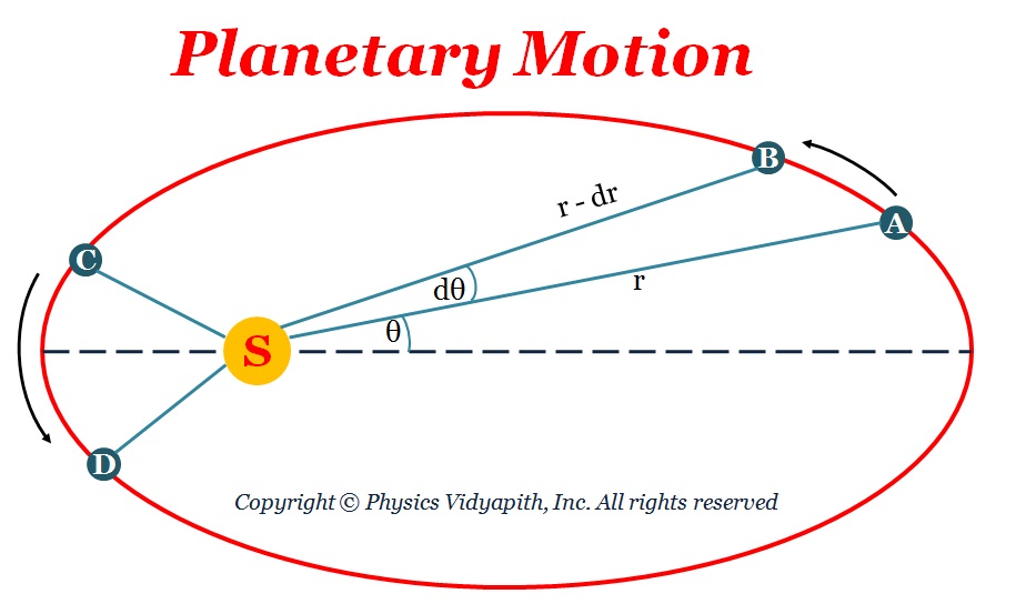
Planetary Motion

From the above figure, A planet is moving around the sun from $A$ to $B$ in a given time interval, and from $C$ to $D$ in the same time interval, then according to the law of areal speed, the areas $ASB$ and $CSD$ will be equal with respect to the same time-interval

Proof →

Let us consider, A planet moves the angle $d\theta$ from $A$ to $B$ in the infinitesimal interval of time $dt$, then the area swept out by radial line $SA$ is

$dA$= Area of the curved $\Delta$ $SAB$

$dA \approx \frac{1}{2} \left( AB \times SA \right)$

$dA \approx \frac{1}{2} \left( r \: d\theta \times r \right)$

$dA \approx \frac{1}{2} \left( r^{2} \: d\theta \right)$

Thus, the instantaneous areal speed of the planets is

$\frac{dA}{dt}=\frac{1}{2} r^{2} \frac{d \theta}{dt}$

$\frac{dA}{dt}=\frac{1}{2} r^{2} \omega \qquad(1)$

Where $\omega$ → The angular speed of the planet.

We know that

$J=I \: \omega$

Where $I$ is the instantaneous moment of inertia of the planet about the Sun $S$.

$J=m \: r^{2} \: \omega \qquad(2)$

Where $m$ is the mass of the planet. Now substitute the value of $r^{2} \: \omega$ from equation $(2)$ in equation $(1)$.

$\frac{dA}{dt}=\frac{J}{2m} \left( Constant \right)$

From the above equation, The areal speed $\frac{dA}{dt}$ of the planet is constant which is Kepler's Second Law. The above equation shows that the angular momentum of the planet is constant. i.e. The angular momentum of any planet is conserved.

Third Law (Law of Periods) →

The square of the time period of one complete revolution of any planet around the sun is directly proportional to the cube of the semi-major axis of its elliptical orbit.

Path of the Planet

Proof →

Let $a$ and $b$ be the semi-major and semi-minor axes of the ellipse, then the area of the ellipse will be $\pi ab$. Let $T$ is the period of one complete revolution of any planet, then

$T=\frac{Area \: of \: the \: ellipse}{Areal \: Speed}$

$T=\frac{\pi a b}{\frac{J}{2m}}$

$T=\frac{2\pi a b m}{J}$

$T^{2}=\frac{4 \pi^{2} a^{2} b^{2} m^{2}}{J^{2}}$

Let $l$ be the semi-latus rectum of the elliptical orbit i.e. $l=\frac{b^{2}}{a}$. Then we get the above equation which can be written as

$T^{2}=\frac{4 \pi^{2} m^{2} a^{3} l }{J^{2}}$

$T^{2} \propto a^{3} $

Where $\frac{4 \pi^{2} m^{2} l }{J^{2}}$ is constant.

From the above equation, It is clear that the larger the distance of a planet from the sun, the larger will be its period of revolution around the sun. The period of revolution of the nearest planet to the sun i.e. Mercury is $88$ days, while that of the faraway planet from the sun i.e. Pluto is $248$ years.

Read More