Difference between sound waves and light waves

Sound Waves:

Sound waves are mechanical waves in nature.

They need a medium to propagate and so cannot be produced in a vacuum.

They can move in all types of mediums as solid liquid or gas whether they are transparent or not.

They propagate in the form of longitudinal waves.

The particle of the medium vibrates along the direction of the propagation and so contraction and rarefaction are formed there.

These are three-dimensional waves.

These waves do not show a polarization effect.

For a normal human being the audible frequency range is $20$ to $20000 Hertz$.

The speed of the sound waves is more in a dense medium than in a rare medium.

Light waves:

light waves are electromagnetic waves in nature.

They don't need any medium and so can produce and propagate in a vacuum.

Their velocity in a vacuum is the maximum of value $3 \times 10^{8} m/s$

They can move in a transparent medium only.

They propagate in the form of transverse waves.

The electric field and magnetic field vibration are perpendicular to the direction of wave propagation.

These wave waves are also three-dimensional waves.

These waves source the polarization effect.

For a normal human being the visible frequency range is $4 \times 10^{18} Hz$ to $8 \times 10^{14} Hz$.

The speed of light is more in rare mediums than in dense ones.

Read More

Momentum wave function for a free particle

A non-relativistic free particle of mass $m$ moving in the positive $x$-direction with speed $v_{x}$ has kinetic energy

$E=\frac{1}{2} m v^{2}_{x}$

and momentum

$p_{x}=mv_{x}$

The energy and momentum are associated with a wave of wavelength $\lambda$ and frequency $\nu$ given by

$\lambda = \frac{h}{p_{x}}$

and

$\nu=\frac{E}{h}$

The propagation constant $k_{x}$ of the wave is

$k_{x}= \frac{2\pi}{\lambda}=\frac{2\pi}{\left(\frac{h}{p_{x}} \right)}=\frac{p_{x}}{\left(\frac{h}{2\pi} \right)}=\frac{p_{x}}{\hbar}$

and the angular frequency $\omega$ is

$\omega = 2\pi \nu = \frac{2\pi E}{\hbar}=\frac{E}{\hbar}$

A plane wave traveling along the $x$ axis in the positive direction may be represented by

$\psi(x,t)=A e^{-i\left(k_{x} \: x - \omega t\right)}$

Now subtitute the value of $\omega$ and $k_{x}$ in above equation then we get

$\psi(x,t)=A e^{i\left( \frac{p_{x}}{\hbar} \: x - \frac{E}{\hbar} \: t\right)}$

$\psi(x,t)=A e^{\frac{i}{\hbar}\left( p_{x} \: x - E \: t\right)}$

The superposition of a number of such waves of propagation number slightly different from an average value traveling simultaneously along the same line in the positive $x$- direction forms a wave packet of small extension. By Fourier's theorem the eave packet may be expressed by

$\psi(x,t) = \frac{1}{\sqrt{2 \pi \hbar}} \int_{-\infty}^{+\infty} A (p_{x}) e^{\frac{i}{\hbar}\left( p_{x} \: x - E \: t \right)} \: \: dp_{x} \qquad(1)$

The function $\psi(x,t)$ is called the momentum wave function for the motion of the free particle in one dimension.

The amplitude $A(p_{x})$ of the $x$-component of the momentum is given by the Fourier tranform

$A(p)=\frac{1}{\sqrt{2 \pi \hbar}} \int_{-\infty}^{+\infty} \psi (x,t) e^{-\frac{i}{\hbar}\left( p_{x} \: x - E \: t \right)} \: \: dx \qquad(2)$

In three dimension the wave function is represented by

$\psi(\overrightarrow{r},t) = \frac{1}{(2 \pi \hbar)^{3/2}} \int_{-\infty}^{+\infty} A (\overrightarrow{p}) e^{\frac{i}{\hbar}\left( \overrightarrow{p} . \overrightarrow{r} - E \: t \right)} \: \: d^{3}\overrightarrow{p} \qquad(3)$

Where $d^{3}\overrightarrow{p}=dp_{x} \: dp_{y} \: dp_{z}$ is the volume element in the momentum space. In equation $(1)$, equation $(2)$ and equation $(3)$ $\frac{1}{\sqrt{2 \pi \hbar}}$ and $\frac{1}{(2 \pi \hbar)^{3/2}}$ are normalization constants.

Read More

Schrodinger's equation for the complex conjugate waves function

Derivation:

The time dependent Schrodinger quation for the wave function function $psi(x,y,z,t)$ is

$-\frac{\hbar^{2}}{2m}\nabla^{2} \psi + V\psi=i\hbar\frac{\partial \psi}{\partial t} \qquad(1)$

Since wave function, $\psi$ is complex quantity i.e.

$\psi=\psi_{1}+i \: \psi_{2} \qquad(2)$

Where $\psi_{1}$ and $\psi_{2}$ are real functions of $x,y,z,t$. Substituting this form for $\psi$ in equation $(1)$, we get

$-\frac{\hbar^{2}}{2m}\nabla^{2} \left( \psi_{1}+i \: \psi_{2} \right) + V\left( \psi_{1}+i \: \psi_{2} \right) \\ \qquad = i\hbar\frac{\partial }{\partial t} \left( \psi_{1}+i \: \psi_{2} \right)$

Equation real and imaginary parts on either side of this equation, we obtain the following two equations:

$-\frac{\hbar^{2}}{2m}\nabla^{2} \psi_{1} + V\psi_{1}=-\hbar\frac{\partial \psi_{2}}{\partial t} \qquad(3)$

$-\frac{\hbar^{2}}{2m}\nabla^{2} \psi_{2} + V\psi_{2}=\hbar\frac{\partial \psi_{1}}{\partial t} \qquad(4)$

Mutiplying equation $(4)$ by $-i$ and adding it to equation $(3)$, we get

$-\frac{\hbar^{2}}{2m}\nabla^{2} \left( \psi_{1} - i \: \psi_{2} \right) + V\left( \psi_{1} - i \: \psi_{2} \right) \\ \qquad = -i\hbar\frac{\partial }{\partial t} \left( \psi_{1} - i \: \psi_{2} \right) \qquad(5)$

The complex conjugate of wave function $\psi^{*}$ is

$\psi^{*}=\psi^{*}_{1} - i \: \psi^{*}_{2} \qquad(6)$

Therefore, The equation $(5)$ can be written as

$-\frac{\hbar^{2}}{2m}\nabla^{2} \psi^{*} + V \psi^{*} =-i \hbar \frac{\partial \psi^{*}}{\partial t}$

This is the equation for complex conjugate wave function $\psi^{*}$.

Read More

Probability Current Density for a free particle in Quantum Mechanics

1.) Derivation of Probability Current Density for a free particle:

Let a particle of mass $m$ is moving in the positive $x$- direction in the region from $x_{1}$ to $x_{2}$.

For the one-dimensional motion of the particle, the wave function is $psi(x,t)$ Let $dA$ be the area of the cross-section of the region.

The probability of finding a particle in the region is

$\int_{x_{1}}^{x_{2}} \psi(x,t) \: \psi^{*}(x,t) \: dx \: dA \qquad(1)$

and the probability density of finding the particle in the region is

$P=\psi(x,t) \: \psi^{*}(x,t) \qquad(2)$

If the probability of finding the particle in the region decreases with time, the rate of decrease of the probability that the particle is in the region from $x_{1}$ to $x_{2}$ per unit area is called the probability current density out of the region. Therefore, the probability current density $S_{2} - S_{1}$ out of the region in the positive $x$-direction is given by

$S_{2} - S_{1} = - \frac{1}{dA} \left[- \frac{d}{dt} \int_{x_{1}}^{x_{2}} P \: dx \: dA \right]$

$S_{2} - S_{1} = - \frac{\partial}{\partial t} \int_{x_{1}}^{x_{2}} P \: dx $

$S_{2} - S_{1} = - \frac{\partial}{\partial t} \int_{x_{1}}^{x_{2}} \psi(x,t) \: \psi^{*}(x,t) \: dx \qquad(3)$

And the probability of current density at position $x$ is

$S = - \frac{\partial}{\partial t} \int \psi(x,t) \: \psi^{*}(x,t) \: dx \qquad(4)$

1.1) Show that: $S = \frac{i \hbar}{2m} \frac{\partial}{\partial x} \left[ \psi^{*} \frac{\partial \psi}{\partial x} - \psi \frac{\partial \psi^{*} }{\partial x} \right]$

Proof:

According to the Schrodinger equation for wave function $\psi(x,t)$ and $\psi^{*}(x,t)$ are

$i \hbar \frac{\partial \psi}{\partial t} =- \frac{\hbar^{2}}{2m} \frac{\partial^{2} \psi}{\partial x^{2}} + V \psi \qquad(1.1.1)$

The complex conjugate of the wave function

$-i \hbar \frac{\partial \psi^{*}}{\partial t} = -\frac{\hbar^{2}}{2m} \frac{\partial^{2} \psi^{*}}{\partial x^{2}} + V \psi^{*} \qquad(1.1.2)$

Multiplying equation $(1.1.1)$ by $\psi^{*}$ and equation $(1.1.2)$ by $\psi$, we get

$i \hbar \psi^{*} \frac{\partial \psi}{\partial t} =- \frac{\hbar^{2}}{2m} \psi^{*} \frac{\partial^{2} \psi}{\partial x^{2}} + \psi^{*} V \psi \quad(1.1.3)$

$-i \hbar \psi \frac{\partial \psi^{*}}{\partial t} = -\frac{\hbar^{2}}{2m} \psi \frac{\partial^{2} \psi^{*}}{\partial x^{2}} + \psi V \psi^{*} \quad(1.1.4)$

Now subtracting equation $(1.1.4)$ and equation $(1.1.3)$, we get

$i \hbar \left( \psi^{*} \frac{\partial \psi}{\partial t} + \psi \frac{\partial \psi^{*}}{\partial t} \right) =-\frac{\hbar^{2}}{2m} \left[ \psi^{*} \frac{\partial^{2} \psi}{\partial x^{2}} - \psi \frac{\partial^{2} \psi^{*}}{\partial x^{2}} \right]$

$i \hbar \frac{\partial}{\partial t} \left( \psi \psi^{*} \right) =-\frac{\hbar^{2}}{2m} \frac{\partial}{\partial x} \left[ \psi^{*} \frac{\partial \psi}{\partial x} - \psi \frac{\partial \psi^{*}}{\partial x} \right]$

$ \frac{\partial}{\partial t} \left( \psi \psi^{*} \right) =\frac{i\hbar}{2m} \frac{\partial}{\partial x} \left[ \psi^{*} \frac{\partial \psi}{\partial x} - \psi \frac{\partial \psi^{*}}{\partial x} \right] \quad(1.1.5)$

We know that

$S = - \frac{\partial}{\partial t} \int \psi(x,t) \: \psi^{*}(x,t) \: dx $

Now substitute the value of equation $(9)$ in the above equation that can be written as

$ S = -\frac{i\hbar}{2m} \int \frac{\partial}{\partial x} \frac{\partial}{\partial x} \left[ \psi^{*} \frac{\partial \psi}{\partial x} - \psi \frac{\partial \psi^{*}}{\partial x} \right] dx $

$ S = -\frac{i\hbar}{2m} \left[ \psi^{*} \frac{\partial \psi}{\partial x} - \psi \frac{\partial \psi^{*}}{\partial x} \right] $

1.2) Show That The probability current density for a free particle is equal to the product of its probability density and its speed.

Proof:

For a free particle that is moving in the positive $x$-axis direction and the momentum $p_{x}$ at position $x$ is given by

$\frac{\hbar}{i} \frac{\partial \psi}{\partial x} = p_{x} \psi$

$ \frac{\partial \psi}{\partial x} = \frac{i}{\hbar} p_{x} \psi \qquad(1.2.1)$

and

$-\frac{\hbar}{i} \frac{\partial \psi^{*}}{\partial x} = p_{x} \psi^{*}$

$ \frac{\partial \psi^{*}}{\partial x} = - \frac{i}{\hbar} p_{x} \psi^{*} \qquad(1.2.2)$

We know that

$ S = -\frac{i\hbar}{2m} \left[ \psi^{*} \frac{\partial \psi}{\partial x} - \psi \frac{\partial \psi^{*}}{\partial x} \right] $

Now substitute the value of equation $(1.2.1)$ and equation $(1.2.2)$ in the above equation, we get

$ S = -\frac{i\hbar}{2m} \left[ \psi^{*} \frac{i}{\hbar} p_{x} \psi + \psi \frac{i}{\hbar} p_{x} \psi^{*}\right] $

$ S = \frac{1}{2m} \left[ \psi^{*} p_{x} \psi + \psi p_{x} \psi^{*}\right] $

$ S = \frac{1}{m} \left( \psi \psi^{*} p_{x} \right)$

$ S = \frac{ p_{x} }{m} \left( \psi \psi^{*}\right) \qquad(1.2.3) $

Now put $p_{x}= m v_{x}$ in equation $(1.2.3)$

$ S = \frac{m v_{x} }{m} \left( \psi \psi^{*}\right)$

$ S = \left( \psi \psi^{*}\right) v_{x}$

Now put $p_{x}= \hbar k_{x}$ in equation $(1.2.3)$

$ S = \frac{ \hbar \: k_{x} }{m} \left( \psi \psi^{*}\right) $

Read More

Ehrenfest's Theorem and Derivation

Ehrenfest's Theorem Statement:

The theorem states that

Quantum mechanics gives the same results as classical mechanics for a particle for which average or expectation values of dynamical quantities are involved.

Proof of theorem:

The proof of the theorem for one-dimensional motion of a particle by showing that

1) $\frac{d \left < x \right >}{dt} = \frac{\left < p_{x} \right > }{m}$

2) $\frac{d \left < p_{x} \right >}{dt} = \left < F_{x} \right >$

1.) To Show that: $\frac{d \left < x \right > }{dt} = \frac{\left < p_{x} \right > }{m}$

Let $x$ is the position coordinate of a particle of mass $m$, at time $t$

The expectation value of position $x$ of a particle is given by

$\left < x \right > = \int_{- \infty}^{+ \infty} \psi^{*} (x,t) . x \: \psi (x,t) dx \qquad (1)$

Differentiating the above equation $(1)$ with respect to $t$

$\frac{d \left < x \right > }{dt} = \int_{- \infty}^{+ \infty} x \frac{\partial (\psi \psi^{*})}{\partial t} dx \qquad(2)$

We know the probablity current density

$\frac{\partial (\psi \psi^{*})}{\partial t} = \frac{i \hbar}{2m} \frac{\partial}{\partial x} \left[ \psi^{*} \frac{\partial \psi}{\partial x} - \psi \frac{\partial \psi^{*} }{\partial x} \right] \qquad(3)$

Now substitute the above eqaution$(3)$ in eqaution $(2)$

$\frac{d \left < x \right > }{dt} = \frac{i \hbar}{2m} \int_{- \infty}^{+ \infty} x \frac{\partial}{\partial x} \left[ \psi^{*} \frac{\partial \psi}{\partial x} - \psi \frac{\partial \psi^{*} }{\partial x} \right] dx $

Integrating the right-hand side by parts of the above equation, we get

$\frac{d \left < x \right > }{dt} = \frac{i \hbar}{2m} \left[ x \left( \psi^{*} \frac{\partial \psi}{\partial x} - \psi \frac{\partial \psi^{*} }{\partial x} \right) \right]^{+\infty}_{-\infty} \\ \qquad - \frac{i \hbar}{2m} \int_{- \infty}^{+ \infty} \left( \psi^{*} \frac{\partial \psi}{\partial x} - \psi \frac{\partial \psi^{*} }{\partial x} \right) dx $

As $x$ approaches either $+ \infty$ or $-\infty$, $\psi$ and $\frac{\partial \psi}{\partial x}$ approach zero, and therefore the first term becomes zero.

Hence we get

$\frac{d \left < x \right > }{dt} = - \frac{i \hbar}{2m} \int_{- \infty}^{+ \infty} \left( \psi^{*} \frac{\partial \psi}{\partial x} - \psi \frac{\partial \psi^{*} }{\partial x} \right) dx \\ \qquad\qquad\qquad\qquad\qquad\qquad ---(4)$

The expectation value of $p_{x}$ is given by

$ \left < p_{x} \right > = \int_{- \infty}^{+ \infty} \psi^{*} \frac{\hbar}{i} \frac{\partial \psi}{\partial x} $

$ \int_{- \infty}^{+ \infty} \psi^{*} \frac{\partial \psi}{\partial x} dx = \frac{i}{\hbar}\left < p_{x} \right > \qquad(5)$

Similarly

$ \int_{- \infty}^{+ \infty} \psi \frac{\partial \psi^{*}}{\partial x} dx = - \frac{i}{\hbar}\left < p_{x} \right > \qquad(6)$

Substituting the values of these integrals in equation $(4)$

$\frac{d \left < x \right > }{dt} = - \frac{i \hbar}{2m} \left[ \frac{i}{\hbar}\left < p_{x} \right > + \frac{i}{\hbar}\left < p_{x} \right >\right] $

$\frac{d \left < x \right > }{dt} = - \frac{\left < p_{x} \right >}{m} \qquad(7)$

This is the first result of Ehrenfest's Theorem.

2) To show that: $\frac{d \left < p_{x} \right >}{dt} = \left < F_{x} \right >$

We know that the expectation value of the momentum $p_{x}$ is given by

$ \left < p_{x} \right > = \int_{- \infty}^{+ \infty} \psi^{*} \frac{\hbar}{i} \frac{\partial \psi}{\partial x} $

$ \left < p_{x} \right > =\frac{\hbar}{i} \int_{- \infty}^{+ \infty} \psi^{*} \frac{\partial \psi}{\partial x} \qquad(8)$

Differentiating the equation $(8)$ with respect to $t$, we get

$\frac{d \left < p_{x} \right >}{dt} = \frac{\hbar}{i} \int_{- \infty}^{+ \infty} \left[ \frac{\partial \psi^{*}}{\partial t} \frac{\partial \psi}{\partial x} + \psi^{*} \frac{\partial^{2} \psi}{\partial x \partial t} \right] $

$\frac{d \left < p_{x} \right >}{dt} = \int_{- \infty}^{+ \infty} \left[-i \hbar \frac{\partial \psi^{*}}{\partial t} \frac{\partial \psi}{\partial x} - i\hbar \psi^{*} \frac{\partial^{2} \psi}{\partial x \partial t} \right] \\ \qquad\qquad\qquad\qquad\qquad\qquad ---(9)$

Now the time-dependent Schrodinger equations for $\psi$ and $\psi^{*}$ are

$i \hbar \frac{\partial \psi}{\partial t} =- \frac{\hbar^{2}}{2m} \frac{\partial^{2} \psi}{\partial x^{2}} + V \psi \qquad(10)$

The complex conjugate of Schrodinger function

$-i \hbar \frac{\partial \psi^{*}}{\partial t} = -\frac{\hbar^{2}}{2m} \frac{\partial^{2} \psi^{*}}{\partial x^{2}} + V \psi^{*} \qquad(11)$

Differentiating the equation $(10)$ with respect to $x$

$i \hbar \frac{\partial^{2} \psi}{\partial x \partial t} = - \frac{\hbar^{2}}{2m} \frac{\partial^{3} \psi}{\partial x^{3}} + \frac{\partial (V \psi)}{\partial x} \qquad(12)$

Now substitute the value of $-i \hbar \frac{\partial \psi^{*}}{\partial t}$ and $i \hbar \frac{\partial^{2} \psi}{\partial x \partial t}$ in the equation $(9)$, we get

$\frac{d \left < p_{x} \right >}{dt} = \int_{- \infty}^{+ \infty} \left[ \left( -\frac{\hbar^{2}}{2m} \frac{\partial^{2} \psi^{*}}{\partial x^{2}} + V \psi^{*} \right) \frac{\partial \psi}{\partial x} - \psi^{*} \left( - \frac{\hbar^{2}}{2m} \frac{\partial^{3} \psi}{\partial x^{3}} + \frac{\partial (V \psi)}{\partial x} \right) \right]$

$\frac{d \left < p_{x} \right >}{dt} = \int_{- \infty}^{+ \infty} \left[-\frac{\hbar^{2}}{2m} \left( \frac{\partial^{2} \psi^{*}}{\partial x^{2}}\frac{\partial \psi}{\partial x} - \psi^{*} \frac{\partial^{3} \psi}{\partial x^{3}} \right) - \left( V \psi^{*} \frac{\partial \psi}{\partial x} - \psi^{*} \frac{\partial (V \psi)}{\partial x} \right) \right] dx$

$\frac{d \left < p_{x} \right >}{dt} = -\frac{\hbar^{2}}{2m} \int_{- \infty}^{+ \infty} \left( \frac{\partial^{2} \psi^{*}}{\partial x^{2}}\frac{\partial \psi}{\partial x} - \psi^{*} \frac{\partial^{3} \psi}{\partial x^{3}} \right) dx + \int_{- \infty}^{+ \infty} \left( V \psi^{*} \frac{\partial \psi}{\partial x} - \psi^{*} \frac{\partial (V \psi)}{\partial x} \right) dx$

$\frac{d \left < p_{x} \right >}{dt} = -\frac{\hbar^{2}}{2m} \int_{- \infty}^{+ \infty} \frac{\partial}{\partial x} \left( \frac{\partial \psi^{*}}{\partial x}\frac{\partial \psi}{\partial x} - \psi^{*} \frac{\partial^{2} \psi}{\partial x^{2}} \right) dx + \int_{- \infty}^{+ \infty} \left( V \psi^{*} \frac{\partial \psi}{\partial x} - \psi^{*} \frac{\partial (V \psi)}{\partial x} \right) dx$

Now put $\frac{\partial (V \psi)}{\partial x}= \left\{ \psi \frac{\partial V }{\partial x}+ V\frac{\partial \psi}{\partial x} \right\}$ in above equation:

$\frac{d \left < p_{x} \right >}{dt} = -\frac{\hbar^{2}}{2m} \int_{- \infty}^{+ \infty} \frac{\partial}{\partial x} \left( \frac{\partial \psi^{*}}{\partial x}\frac{\partial \psi}{\partial x} - \psi^{*} \frac{\partial^{2} \psi}{\partial x^{2}} \right) dx + \int_{- \infty}^{+ \infty} \left( V \psi^{*} \frac{\partial \psi}{\partial x} - \psi^{*} \left\{ \psi \frac{\partial V }{\partial x}+ V\frac{\partial \psi}{\partial x} \right\} \right) dx$

$\frac{d \left < p_{x} \right >}{dt} = -\frac{\hbar^{2}}{2m} \left[ \frac{\partial \psi^{*}}{\partial x}\frac{\partial \psi}{\partial x} - \psi^{*} \frac{\partial^{2} \psi}{\partial x^{2}} \right]_{- \infty}^{+ \infty} + \int_{- \infty}^{+ \infty} \left( V \psi^{*} \frac{\partial \psi}{\partial x} - \psi^{*} \left\{ \psi \frac{\partial V }{\partial x}+ V\frac{\partial \psi}{\partial x} \right\} \right) dx$

As $x$ approaches either $+ \infty $ or $-\infty$ and $\frac{\partial \psi}{\partial x}$ is zero. Therefore the first term of the above equation on the right-hand side will be zero.

$\frac{d \left < p_{x} \right >}{dt} = \int_{- \infty}^{+ \infty} \left( V \psi^{*} \frac{\partial \psi}{\partial x} - \psi^{*} \left\{ \psi \frac{\partial V }{\partial x}+ V\frac{\partial \psi}{\partial x} \right\} \right) dx$

$\frac{d \left < p_{x} \right >}{dt} = \int_{- \infty}^{+ \infty} \left( V \psi^{*} \frac{\partial \psi}{\partial x} - \psi \frac{\partial V }{\partial x} \psi^{*} - V \psi^{*} \frac{\partial \psi}{\partial x} \right) dx$

$\frac{d \left < p_{x} \right >}{dt} = \int_{- \infty}^{+ \infty} - \psi \frac{\partial V }{\partial x} \psi^{*} dx$

$\frac{d \left < p_{x} \right >}{dt} = - \int_{- \infty}^{+ \infty} \psi \frac{\partial V }{\partial x} \psi^{*} dx$

$\frac{d \left < p_{x} \right >}{dt} = -\left < \frac{\partial V }{\partial x} \right > $

Here the $\left < \frac{\partial V }{\partial x} \right >$ is the average value or expectation value of potential gradient and the negative value of the potential gradient is equal to the average value or expectation value of force $\left < F_{x} \right >$ along the $x$ direction.

$\frac{d \left < p_{x} \right >}{dt} = \left < F_{x} \right > $

This is the second result of Ehrenfest theorem and it represents Newton's second law of motion. Thus if the expectation values of dynamical quantities for a particle are, considered, quantum mechanics given the equations of classical mechanics.

Read More

Eigen value of the momentum of a particle in one dimension box or infinite potential well

Equation of eigen value of the momentum of a particle in one dimension box:

The eigen value of the momentum $P_{n}$ of a particle in one dimension box moving along the x-axis is given by

$P^{2}_{n} = 2 m E_{n}$

$P^{2}_{n} = 2 m \frac{n^{2} \pi^{2} \hbar^{2}}{2 m L^{2}} \qquad \left( \because E_{n}= \frac{n^{2} \pi^{2} \hbar^{2}}{2 m L^{2}} \right)$

$P^{2}_{n} = \frac{n^{2} \pi^{2} \hbar^{2}}{L^{2}}$

$P_{n} = \pm \frac{n \pi \hbar}{L}$

$P_{n} = \pm \frac{n h}{2L} \qquad \left( \hbar = \frac{h}{2 \pi} \right)$

The $\pm$ sign indicates that the particle is moving back and forth in the infinite potential box.

The above equation shows that eigen value of the momentum of the particle is discrete and the difference between the momentum corresponding to two consecutive energy levels is always constant and equal to $\frac{h}{2L}$

Read More

Electric field intensity due to uniformly charged solid sphere (Conducting and Non-conducting)

A.) Electric field intensity at different points in the field due to the uniformly charged solid conducting sphere:

Let us consider, A solid conducting sphere that has a radius $R$ and charge $+q$ is distributed on the surface of the sphere in a uniform manner. Now find the electric field intensity at different points due to the solid-charged conducting sphere. These different points are: 1.) Electric field intensity outside the solid conducting sphere
2.) Electric field intensity on the surface of the solid conducting sphere
3.) Electric field intensity inside the solid conducting sphere

1.) Electric field intensity outside the solid conducting sphere:

If $O$ is the center of solid conducting spherical then the electric field intensity outside of the sphere can be determined by the following steps →

1.) First, take the point $P$ outside the sphere
2.) Draw a spherical surface of radius r which passes through point $P$. This hypothetical surface is known as the Gaussian surface.
3.) Now take a small area $\overrightarrow {dA} $ around point $P$ on the Gaussian surface to find the electric flux passing through it.
4.) Now find the direction between the electric field vector and a small area vector.

Due to uniform charge distribution, the electric field intensity will be the same at every point on the Gaussian surface. So from the figure,

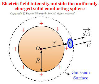The direction of electric field intensity on the Gaussian surface is radially outward which is in the direction of the area vector of the Gaussian surface. i.e. ($\theta=0^{\circ}$). Here $\overrightarrow {dA}$ is a small area around point $P$ so the small electric flux $d\phi_{E}$ will pass through this small area $\overrightarrow {dA}$. so this flux can be found by applying Gauss's law in question given below:

$ d\phi_{E}= \overrightarrow {E}\cdot \overrightarrow{dA}$

$ d\phi_{E}= E\:dA\: cos\: 0^{\circ} \quad \left \{\because \theta=0^{\circ} \right \}$

$ d\phi_{E}= E\:dA \quad (1) \quad \left \{\because cos\:0^{\circ}=1 \right \}$

The electric flux passes through the entire Gaussian surface, So integrate the equation $(1)$ →

$ \oint d\phi_{E}= \oint E\:dA $

$\phi_{E}=\oint E\:dA\qquad (2)$

According to Gauss's law:

$ \phi_{E}=\frac{q}{\epsilon_{0}}\qquad (3)$

From equation $(2)$ and equation $(3)$, we can write as

$ \frac{q}{\epsilon_{0}}=\oint E\:dA$

$ \frac{q}{\epsilon_{0}}= E\oint dA$

Now substitute the area of the entire Gaussian spherical is $\oint {dA}=4\pi r^{2}$ in the above equation. So the above equation can be written as:

$ \frac{q}{\epsilon_{0}}= E(4\pi r^{2})$

$ E=\frac{1}{4\pi \epsilon_{0}}\frac{q}{r^{2}}$

From the above equation, we can conclude that the behavior of the electric field at the external point due to the uniformly charged solid conducting sphere is the same as the entire charge is placed at the center, point charge

If the surface charge density is $\sigma$, Then the total charge $q$ on the surface of a solid conducting sphere is→

$ q=4\pi R^{2}\: \sigma$

Substitute this value of charge $q$ in the above equation, so we can write the equation as:

$ E=\frac{1}{4\pi \epsilon_{0}}\frac{4\pi R^{2}\: \sigma}{r^{2}}$

$ E=\frac{\sigma}{\epsilon_{0}}\frac{R^{2}}{r^{2}}$

This equation describes the electric field intensity at the external point of the solid conducting sphere.

2.) Electric field intensity on the surface of the solid conducting sphere:

If point $P$ is placed on the surface of the solid conducting sphere i.e. ($r=R$). so electric field intensity on the surface of the solid conducting sphere can be found by putting $r=R$ in the formula of electric field intensity at the external point of the solid conducting sphere:

$ E=\frac{1}{4\pi \epsilon_{0}}\frac{q}{R^{2}}$

$ E=\frac{\sigma}{\epsilon_{0}}$

3.) Electric field intensity inside the solid conducting sphere:

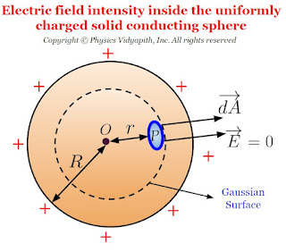If point $P$ is placed inside the solid conducting sphere then electric field intensity will be zero because the charge is distributed uniformly on the surface of the solid sphere and there will not be any charge on the Gaussian surface. So the electric flux will be zero inside the solid sphere. i.e.

$ \phi_{E}=\oint E\:dA$

$ 0=E\oint dA \qquad\quad \left \{ \because \phi_{E}=0 \right \}$

$ E=0$

Electric field intensity distribution with distance for Conducting Solid Sphere:

Electric field intensity distribution with distance shows that the electric field is maximum on the surface of the sphere and zero inside the sphere. Electric field intensity distribution outside the sphere reduces with the distance according to $E=\frac{1}{r^{2}}$.

B.) Electric field intensity at different points in the field due to the uniformly charged solid non-conducting sphere:

Let us consider, A solid non-conducting sphere of radius R in which $+q$ charge is distributed uniformly in the entire volume of the sphere. So electric field intensity at a different point due to the solid charged non-conducting sphere:

1. Electric field intensity outside the solid non-conducting sphere
2. Electric field intensity on the surface of the solid non-conducting sphere
3. Electric field intensity inside the non-solid conducting sphere

1.) Electric field intensity outside the solid non-conducting sphere:

Let us consider, An external point $P$ which is at a distance $r$ from the center point $O$ of the sphere. The electric flux is radially outward in the sphere. So the direction of the electric field vector and the small area vector will be in the same direction i.e. ($\theta =0^{\circ}$). Here $\overrightarrow {dA}$ is a small area, the small amount of electric flux will pass through this area i.e. →

$ d\phi_{E}= \overrightarrow {E}\cdot \overrightarrow{dA}$

$ d\phi_{E}= E\:dA\: cos\: 0^{\circ} \quad \left \{\because \theta=0^{\circ} \right \}$

$ d\phi_{E}= E\:dA \qquad (1) \quad \left \{\because cos\:0^{\circ}=1 \right \}$

The electric flux passes through the entire Gaussian surface, So integrate the equation $(1)$ →

$ \phi_{E}=\oint E\:dA\qquad (2)$

According to Gauss's law:

$ \phi_{E}=\frac{q}{\epsilon_{0}}\qquad (3)$

From equation (1) and equation (2), we can write as

$ \frac{q}{\epsilon_{0}}=\oint E\:dA$

$ \frac{q}{\epsilon_{0}}= E\oint dA$

Now substitute the area of the entire Gaussian spherical surface is $\oint {dA}=4\pi r^{2}$ in the above equation. So the above equation can be written as:

$ \frac{q}{\epsilon_{0}}= E(4\pi r^{2})$

$ E=\frac{1}{4\pi \epsilon_{0}}\frac{q}{r^{2}}$

From the above equation, we can conclude that the behavior of the electric field at the external point due to the uniformly charged solid non-conducting sphere is the same as the point charge i.e. like the entire charge is placed at the center.

Since the sphere is a non-conductor so the charge is distributed in the entire volume of the sphere. So charge distribution can calculate by volume charge density →

$q=\frac{4}{3} \pi R^{3} \rho $

Substitute this value of charge $q$ in the above equation, so we can write the equation as:

$ E=\frac{1}{4\pi \epsilon_{0}}\frac{4\pi R^{3}\: \rho}{3r^{2}}$

$ E=\frac{\rho}{\epsilon_{0}}\frac{R^{3}}{3r^{2}}$

This equation describes the electric field intensity at the external point of the solid non-conducting sphere.

2.) Electric field intensity on the surface of the solid non-conducting sphere:

If point $P$ is placed on the surface of a solid non-conducting sphere i.e. ($r=R$). so electric field intensity on the surface of a solid non-conducting sphere can be found by putting $r=R$ in the formula of electric field intensity at the external point of the solid non-conducting sphere:

$ E=\frac{1}{4\pi \epsilon_{0}}\frac{q}{R^{2}}$

$ E=\frac{\rho R}{3\epsilon_{0}}$

3.) Electric field intensity inside the solid non-conducting sphere:

If point $P$ is placed inside the sphere and the distance from the origin $O$ is $r$, the electric flux which is passing through the Gaussian surface

$ \phi_{E}= E.4\pi r^{2}$

Where $\phi_{E}=\frac{q'}{\epsilon_{0}}$

$ \frac{q'}{\epsilon_{0}}=E.4\pi r^{2}$

Where $q'$ is part of charge $q$ which is enclosed with Gaussian Surface

$ E=\frac{1}{4 \pi \epsilon_{0}} \frac{q'}{r^{2}} \qquad \qquad (4)$

The charge is distributed uniformly in the entire volume of the sphere so volume charge density $\rho$ will be the same as the entire solid sphere i.e.

$ \rho=\frac{q}{\frac{4}{3}\pi R^{3}}=\frac{q'}{\frac{4}{3}\pi r^{3}}$

$ \frac{q}{\frac{4}{3}\pi R^{3}}=\frac{q'}{\frac{4}{3}\pi r^{3}}$

$ q'=q\frac{r^{3}}{R^{3}}$

$ q'=q\left (\frac{r}{R} \right)^{3}$

Put the value of $q'$ in equation $(4)$, so

$ E=\frac{1}{4\pi \epsilon_{0}}\frac{q}{r^{2}}\left(\frac{r}{R} \right)^{3}$

$ E=\frac{1}{4\pi \epsilon_{0}}\frac{qr}{R^{3}}$

Where $q=\frac{4}{3} \pi R^{3} \rho $. So above equation can be written as:

$ E=\frac{1}{4\pi \epsilon_{0}}\frac{\frac{4}{3} \pi R^{3} \rho r}{R^{3}}$

$E=\frac{ \rho r}{3 \epsilon_{0}}$

Electric field intensity distribution with distance for non-conducting Solid Sphere:

Electric field intensity distribution with distance shows that the electric field is maximum on the surface of the sphere and zero at the center of the sphere. Electric field intensity distribution outside the sphere reduces with the distance according to $E=\frac{1}{r^{2}}$.

Read More