The electric potential energy of an electric dipole in the uniform electric field

Derivation of the electric potential energy of an electric dipole in the uniform electric field:

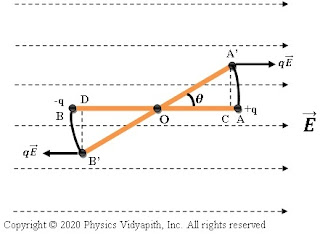
Let us consider an electric dipole $AB$, which is made up of two charges $q_1$ and $q_2$, which are placed at a distance of $l$ in the electric field $E$. So force acting on each charge due to the electric field will be $qE$. If the dipole gets rotated a small-angle $d\theta$ against the torque acting on it in the uniform electric field $E$ then the small work done is

$dW=\tau. d\theta \qquad (1)$

Force of moment on an electric Dipole

The torque (i.e moment of force) on an electric dipole in a uniform electric field

$ \tau=p.E\:sin\theta$

Now substitute the value of $\tau$ in equation $(1)$. So work done

$ dW=p.E\:sin\theta.d\theta$

If the dipole rotate the angle from $\theta_{1}$ to angle $\theta_{2}$ then workdone

$\int_{W_{1}}^{W_{2}}dW=p.E\int_{\theta_{1}}^{\theta_{2}}sin\theta \: d\theta$

$ W_{2}-W_{1}=p.E\left[-cos\theta \right]_{\theta_{1}}^{\theta_{2}}$

$ \Delta W= p.E \left( cos\theta_{1}-cos\theta_{2} \right)\qquad\qquad (2)$

This work is stored in the form of the electric potential energy of an electric dipole in the electric field. So

$U=\Delta W$

$U=p.E \left( cos\theta_{1}-cos\theta_{2} \right)$

If the electric dipole rotates from $0^{\circ}$ (when the direction of electric dipole moment $p$ is aligned in the direction of the electric field $E$) to an angle $\theta$ in the electric field i.e $\theta_{1}=0^{\circ}$ and $\theta_{2}=\theta$ then the electric potential energy of dipole in a uniform electric field

$U=p.E (1-cos\theta)$

Case-(I) If $\theta=0^{\circ}$ i.e It is stable equilibrium position then

$U_{min}=0$

Case-(II) If $\theta=90^{\circ}$ i.e Position of zero energy then

$U=pE$

Case-(III) If $\theta=180^{\circ}$ i.e It is unstable equilibrium position then

$U_{max}=2pE$

Read More

de-Broglie Concept of Matter wave

Louis de-Broglie thought that similar to the dual nature of light, material particles must also possess the dual character of particle and wave. This means that material particles sometimes behave as particle nature and sometimes behave like a wave nature.

According to de-Broglie –

A moving particle is always associated with a wave, called as de-Broglie matter-wave, whose wavelengths depend upon the mass of the particle and its velocity.

According to Planck’s theory of radiation–

$E=h\nu \qquad(1) $

Where
h – Planck’s constant
$\nu $ - frequency

According to Einstein’s mass-energy relation –

$E=mc^ {2} \qquad (2)$

According to de Broglie's hypothesis equation $ (1)$ and equation $(2)$ can be written as –

$mc^ {2} = h \nu$

$mc^ {2} = \frac{hc}{\lambda }$

$\lambda =\frac{h}{mc}\qquad(3) $

$\lambda =\frac{h}{P}$

Where $P$ –Momentum of Photon

Similarly from equation $(3)$ the expression for matter waves can be written as

$\lambda=\frac{h}{mv}=\frac{h}{P}\qquad(4)$

Here $P$ is the momentum of the moving particle.

1.) de-Broglie Wavelength in terms of Kinetic Energy

$K=\frac{1}{2} mv ^{2}$

$K=\frac{m^{2}v^{2}}{2m}$

$K=\frac{P^{2}}{2m}$

$P=\sqrt{2mK}$

Now substitute the value of $P$ in equation $ (4)$ so

$\lambda =\frac{h}{\sqrt{2mK}} \qquad (5)$

2.) de-Broglie Wavelength for a Charged particle

The kinetic energy of a charged particle is $K = qv$

Now substitute the value of $K$ in equation$(5)$ so

$\lambda =\frac{h}{\sqrt{2mqv}}$

3.) de-Broglie Wavelength for an Electron

The kinetic energy of an electron

$K=ev$

If the relativistic variation of mass with a velocity of the electron is ignored then $m=m_{0}$ wavelength

$\lambda =\frac{h}{\sqrt{2m_{0}ev}}$

So wavelength of de-Broglie wave associated with the electron in non-relativistic cases

4.) de-Broglie wavelength for a particle in Thermal Equilibrium

For a particle of mass $m$ in thermal equilibrium at temperature $T@

$K=\frac{3}{2}kT$

Where $K$ – Boltzmann Constant

$\lambda =\frac{h}{\sqrt{2m.\frac{3}{2}kt}}$

$\lambda =\frac{h}{\sqrt{3mKT}}$

Properties of matter wave →

1. Matter waves are generated only if the material's particles are in motion.


2. Matter-wave is produced whether the particles are charged or uncharged.
3. The velocity of the matter wave is constant; it depends on the velocity of material particles.


4. For the velocity of a given particle, the wavelength of matter waves will be shorter for a particle of large mass and vice-versa.


5. The matter waves are not electromagnetic waves.


6. The speed of matter waves is greater than the speed of light.
   
   
   According to Einstein’s mass-energy relation
   
   
   $E=mc^{2}$
   
   
   $h\nu = mc^{2}$
   
   
   $\nu =\frac{mc^{2}}{h}$
   
   
   Where $\nu$ is the frequency of matter-wave.
   
   
   We know that the velocity of matter-wave
   
   
   $ u =\nu \lambda $
   Substitute the value of $\nu$ in the above equation
   
   
   $u =\frac{mc^{2}}{h}. \lambda $
   $u =\frac{mc^{2}}{h} . \frac{h}{mv}$
   
   

   $u =\frac{c^{2}}{v}$

   
   
   Where $v$ → particle velocity which is less than the velocity of light.


7. The wave and particle nature of moving bodies can never be observed simultaneously.

Read More

Group velocity is equal to particle velocity

Prove that: Group velocity is equal to Particle Velocity

Solution:

We know that group velocity

$V_{g}=\frac{d\omega}{dk}$

$V_{g}=\frac{d(2\pi\nu )}{d(\frac{2\pi }{\lambda })} \qquad \left(k=\frac{2\pi}{\lambda} \right)$

$V_{g}=\frac{d\nu}{d(\frac{1}{\lambda })}$

$\frac{1}{V_{g}}=\frac{d( \frac{1}{\lambda })}{d\nu}\qquad(1)$

We know that the total energy of the particle is equal to the sum of kinetic energy and potential energy. i.e

$E=K+V$

Where

$K$ – kinetic energy
$V$ – Potential energy

$E=\frac{1}{2} mv^{2}+V$

$E-V=\frac{1}{2}\frac{(mv)^2}{m}$

$E-V=\frac{1}{2m }(mv)^2$

$2m(E-V)=(mv)^2$

$mv=\sqrt{2m(E-V)}$

According to de-Broglie wavelength-

$\lambda =\frac{h}{mv}$

$\lambda =\frac{h}{\sqrt{2m(E-V)}}$

$\frac{1}{\lambda} =\frac{\sqrt{2m(E-V)}}{h}\qquad(3)$

Now put the value of $\frac{1}{\lambda }$ in equation$(1)$

$\frac{1}{V_{g}} =\frac{d}{dv}[\frac{{2m(E-V)}^\tfrac{1}{2}}{h}]$

$\frac{1}{V_{g}} =\frac{d}{dv}[\frac{{2m(h\nu -V)}^\tfrac{1}{2}}{h}]$

$\frac{1}{V_{g}} =\frac{1}{2h}[{2m(h\nu -V)}]^{\tfrac{-1}{2}}{2m.h}$

$\frac{1}{V_{g}} =\frac{1}{2h}[{2m(E -V)}]^{\tfrac{-1}{2}}{2m.h} \qquad \left(\because E=h\nu \right) $

$\frac{1}{V_{g}} =\frac{m}{mv}$     {from equation $(2)$}

$V_{g}=V$

Thus, the above equation shows that group velocity is equal to particle velocity.

Read More

Principle, Construction and Working of Venturimeter

Principle of Venturimeter:

It is a device for measuring the rate of liquid flow through pipes. Its principle and workings are based on Bernoulli's theorem and equation.

Construction:

It consists of two identical coaxial tubes, $X$ and $Z$, connected by a narrow coaxial tube $Y$. Two vertical tubes $P$ and $Q$ are mounted on tubes $X$ and $Y$ to measure the pressure of the liquid that flows through pipes. As shown in the figure below.

Working and Theory:

Connect this venturimeter horizontally to the pipe through which the liquid is flowing and note down the difference of liquid columns in tubes $P$ and $E$. Let the difference be $h$.

Let us consider that an incompressible and non-viscous liquid flows in streamlined motion through a tube $X$,$Y$, and $Z$ of a non-uniform cross-section.

Now Consider:

The cross-section's area of tube $X$ = $A_{1}$
The cross-section's area of tube $Y$ = $A_{2}$

The velocity of fluid per second (i.e., equal to distance) at the cross-section of tube $X$ = $v_{1}$
The velocity of fluid per second (i.e., equal to distance) at the cross-section of tube $Y$ = $v_{2}$

The fluid's pressure at cross-section of tube $X$ = $P_{1}$
The fluid's pressure at cross-section of tube $Y$ = $P_{2}$

Now the change in pressure on tube $P$ and $Q$:

$P_{1}-P_{2}=\rho g h \qquad(1)$

Where $\rho$ is the density of the liquid.

According to the principle of continuity:

$A_{1} v_{1} = A_{2} v_{2} = \frac{m}{\rho}= V  \quad(2)$

Where $V$ is the volume of the liquid flowing per second through the pipe. Then from equation $(2)$

$\left.\begin{matrix} v_{1}=\frac{V}{A_{1}} \\ v_{2}=\frac{V}{A_{2}} \end{matrix}\right\} \qquad(3)$

Now apply Bernoulli's Theorem for horizontal flow (i.e, $h_{1}=h_{2}$) in a verturimeter.

$P_{1} + \frac{1}{2} \rho v_{1}^{2} = P_{2} + \frac{1}{2}\rho v_{2}^{2} $

$P_{1} - P_{2} = \frac{1}{2}\rho v_{2}^{2} - \frac{1}{2} \rho v_{1}^{2} $

$P_{1} - P_{2} = \frac{1}{2}\rho \left( v_{2}^{2} - v_{1}^{2} \right) \qquad(4) $

Now from equation $(1)$ and equation $(4)$, we get

$\rho g h = \frac{1}{2}\rho \left( v_{2}^{2} - v_{1}^{2} \right)$

$g h = \frac{1}{2} \left( v_{2}^{2} - v_{1}^{2} \right)$

Now substitute the value of $v_{1}$ and $v_{2}$ from equation $(3)$ in above equation

$g h = \frac{1}{2} \left( \frac{V^{2}}{A^{2}_{2}} - \frac{V^{2}}{A^{2}_{1}} \right)$

$g h = \frac{V^{2}}{2} \left( \frac{1}{A^{2}_{2}} - \frac{1}{A^{2}_{1}} \right)$

$g h = \frac{V^{2}}{2} \left( \frac{ A^{2}_{1} - A^{2}_{2} }{A^{2}_{1} A^{2}_{2}} \right)$

$V^{2} = \frac{2 g h A^{2}_{1} A^{2}_{2}}{A^{2}_{1} - A^{2}_{2}}$

$V = A_{1} A_{2} \sqrt{\frac{2 g h }{A^{2}_{1} - A^{2}_{2}}}$

Hence flow rate of liquid can be calculated by measuring $h$, since $A_{1}$ and $A_{2}$ are known for the given venturimeter.

Read More

Solution of electromagnetic wave equations in conducting media

The electromagnetic wave equations in conducting media:

For electric field vector:

$ \nabla^{2}.\overrightarrow{E}-\mu \epsilon\frac{\partial^{2} \overrightarrow{E}}{\partial t^{2}} - \sigma \mu \frac{\partial \overrightarrow{E}}{\partial t}=0 \qquad(1)$

For magnetic field vector:

$\nabla^{2}.\overrightarrow{B} - \mu \epsilon \frac{\partial^{2} B}{\partial t^{2}}-\sigma \mu \frac{\partial \overrightarrow{B}}{\partial t}=0 \qquad(2)$

The wave equation of electric field vector:

$\overrightarrow{E}(\overrightarrow{r},t)=E_{\circ} e^{i(\overrightarrow{k}. \overrightarrow{r} - \omega t)} \qquad(3)$

The wave equation of magnetic field vector:

$\overrightarrow{B}(\overrightarrow{r},t)=B_{\circ} e^{i(\overrightarrow{k}. \overrightarrow{r} - \omega t)} \qquad(4)$

Now the solution of electromagnetic wave for electric field vector.

Differentiate with respect to $t$ of equation $(3)$

$\frac{\partial \overrightarrow{E}}{\partial t}=i \omega E_{\circ} e^{i(\overrightarrow{k}. \overrightarrow{r} - \omega t)}$

Again differentiate with respect to $t$ of the above equation:

$\frac{\partial^{2} \overrightarrow{E}}{\partial t^{2}}=i^{2} \omega^{2} E_{\circ} e^{i(\overrightarrow{k}. \overrightarrow{r} - \omega t)}$

$\frac{\partial^{2} \overrightarrow{E}}{\partial^{2} t}=- \omega^{2} \overrightarrow{E}(\overrightarrow{r},t)$

Now substitute the value of the above equation in equation$(1)$

$\nabla^{2} \overrightarrow{E}=-\omega^{2} \mu \epsilon \overrightarrow{E} - i \omega \mu \sigma \overrightarrow{E}$

$\nabla^{2} \overrightarrow{E}=- \left( \omega^{2} \mu \epsilon + i \omega \mu \sigma \right) \overrightarrow{E}$

This is the solution of the electromagnetic wave equation in conducting media for the electric field vector.

Now component form of the above equation:

$(\frac{\partial^{2}}{\partial x^{2}} + \frac{\partial^{2}}{\partial y^{2}} +\frac{\partial^{2}}{\partial z^{2}})(\hat{i}E_{x}+\hat{j}E_{y}+\hat{k}E_{z}) \\ =- \left( \omega^{2} \mu \epsilon + i \omega \mu \sigma \right)(\hat{i}E_{x}+\hat{j}E_{y}+\hat{k}E_{z}) \qquad(5)$

If the wave is propagating along $z$ direction. Then for uniform-plane electromagnetic waves-

$\frac{\partial}{\partial x}=\frac{\partial}{\partial y}=0$

$\frac{\partial^{2}}{\partial x^{2}}=\frac{\partial^{2}}{\partial y^{2}}=0$

$E_{z}=0$

Now the equation $(5)$ can be written as:

$\frac{\partial^{2}}{\partial x^{2}} (\hat{i}E_{x}+\hat{j}E_{y}) \\ =- \left( \omega^{2} \mu \epsilon + i \omega \mu \sigma \right)(\hat{i}E_{x}+\hat{j}E_{y})$

Now separate the above equation in $x$ and $y$ components so

$\left.\begin{matrix} \frac{\partial^{2} E_{x}}{\partial z^{2}}=- \left( \omega^{2} \mu \epsilon + i \omega \mu \sigma \right) E_{x} \\ \frac{\partial^{2}E_{y}}{\partial z^{2}} =- \left( \omega^{2} \mu \epsilon + i \omega \mu \sigma \right) E_{y} \end{matrix}\right\} \quad(6)$

The solution of electromagnetic wave for magnetic field vector can find out by following the above method.

Therefore $x$ and $y$ components of the solution of the electromagnetic wave equation for magnetic field vector can be written as. i.e.

$\left.\begin{matrix} \frac{\partial^{2} B_{x}}{\partial z^{2}}=- \left( \omega^{2} \mu \epsilon + i \omega \mu \sigma \right) B_{x} \\ \frac{\partial^{2}B_{y}}{\partial z^{2}} =- \left( \omega^{2} \mu \epsilon + i \omega \mu \sigma \right) B_{y} \end{matrix}\right\} \quad(7)$

In the solution of electromagnetic wave equation $(6)$ and equation $(7)$. The term $\left( \omega^{2} \mu \epsilon + i \omega \mu \sigma \right)$ is equal to $k_{z}^{2}$. It is known as propagation constant $k_{z}$. Then

$k_{z}^{2}=\left( \omega^{2} \mu \epsilon + i \omega \mu \sigma \right) \qquad(8)$

The propagation constant is the complex quantity so

$k_{z}=\alpha+i \beta \qquad(9)$

Now from equation $(8)$ and equation $(9)$

$\left(\alpha+i \beta \right)^{2}=\left( \omega^{2} \mu \epsilon + i \omega \mu \sigma \right)$

$\alpha^{2} - \beta^{2} +2 i \alpha \beta =\left( \omega^{2} \mu \epsilon + i \omega \mu \sigma \right)$

Now separate the real and imaginary terms:

$Real \: Term \rightarrow \alpha^{2} - \beta^{2} = \omega^{2} \mu \epsilon \quad (10)$

$Imaginary \: Term \rightarrow 2 \alpha \beta = \omega \mu \sigma \quad (11)$

On solving the equation $(10)$ and equation $(11)$

$\alpha= \omega \sqrt{\frac{\mu \epsilon}{2}} \left[ 1 + \left\{ 1+ \left( \frac{\sigma}{\epsilon \omega} \right)^{2} \right\}^{1/2} \right]^{1/2} \quad(12)$

$\beta= \omega \sqrt{\frac{\mu \epsilon}{2}} \left[ \left\{ 1+ \left( \frac{\sigma}{\epsilon \omega} \right)^{2} \right\}^{1/2} -1 \right]^{1/2} \quad(13)$

The wave equation $(3)$ of the electric field vector also can be written as:

$\overrightarrow{E}(\overrightarrow{r},t)=E_{\circ} e^{-\beta \overrightarrow{r}}e^i{(\alpha \overrightarrow{r} - \omega t)} \qquad(14)$

The above equation has an additional term $e^{-\beta \overrightarrow{r}}$ compared to the purely harmonic solution.

Where
$\alpha \rightarrow$ Attenuation Constant
$\beta \rightarrow$ Absorption Coefficient and Phase Constant

Read More

Electromagnetic Wave Equation in Conducting Media (i.e. Lossy dielectric or Partially Conducting)

Maxwell's Equations: Maxwell's equation of the electromagnetic wave is a collection of four equations i.e. Gauss's law of electrostatic, Gauss's law of magnetism, Faraday's law of electromotive force, and Ampere's Circuital law. Maxwell converted the integral form of these equations into the differential form of the equations. The differential form of these equations is known as Maxwell's equations.

1. $\overrightarrow{\nabla}. \overrightarrow{E}= \frac{\rho}{\epsilon_{0}}$


2. $\overrightarrow{\nabla}. \overrightarrow{B}=0$


3. $\overrightarrow{\nabla} \times \overrightarrow{E}=-\frac{\partial \overrightarrow{B}}{\partial t}$


4. $\overrightarrow{\nabla} \times \overrightarrow{B}= \mu \overrightarrow{J}$
   
   
   Modified form:
   
   
   $\overrightarrow{\nabla} \times \overrightarrow{B}= \mu \overrightarrow{J}+\mu \epsilon \frac{\partial \overrightarrow{E}}{\partial t}$

For Conducting Media:

Current density $(\overrightarrow{J}) = \sigma \overrightarrow{E} $
Volume charge distribution $(\rho)=0$
Permittivity of Conducting Media= $\epsilon$
Permeability of Conducting Media=$\mu$

Now, Maxwell's equation for Conducting Media:

$\overrightarrow{\nabla}. \overrightarrow{E}=0 \qquad(1)$
$\overrightarrow{\nabla}. \overrightarrow{B}=0 \qquad(2)$
$\overrightarrow{\nabla} \times \overrightarrow{E}=-\frac{\partial \overrightarrow{B}}{\partial t} \qquad(3)$
$\overrightarrow{\nabla} \times \overrightarrow{H}= \overrightarrow{J}$

Modified form for Conducting Media:

$\overrightarrow{\nabla} \times \overrightarrow{B}= \mu \overrightarrow{J}+\mu \epsilon \frac{\partial \overrightarrow{E}}{\partial t}$

$\overrightarrow{\nabla} \times \overrightarrow{B}= \mu \sigma \overrightarrow{E}+ \mu \epsilon \frac{\partial \overrightarrow{E}}{\partial t} \qquad(4)$

Now, On solving Maxwell's equation for conducting media i.e perfect dielectric and lossless media, gives the electromagnetic wave equation for conducting media. The electromagnetic wave equation has both an electric field vector and a magnetic field vector. So Maxwell's equation for conducting medium gives two equations for electromagnetic waves i.e. one is for electric field vector($\overrightarrow{E}$) and the second is for magnetic field vector ($\overrightarrow{H}$).

Electromagnetic wave equation for conducting media in terms of $\overrightarrow{E}$:

Now from equation $(3)$

$\overrightarrow{\nabla} \times \overrightarrow{E}=-\frac{\partial \overrightarrow{B}}{\partial t} $

Now take the curl on both sides of the above equation$

$\overrightarrow{\nabla} \times (\overrightarrow{\nabla} \times \overrightarrow{E})=-\overrightarrow{\nabla} \times \frac{\partial \overrightarrow{B}}{\partial t} $

$(\overrightarrow{\nabla}. \overrightarrow{E}).\overrightarrow{\nabla} - (\overrightarrow{\nabla}. \overrightarrow{\nabla}).\overrightarrow{E}=-\frac{\partial}{\partial t} (\overrightarrow{\nabla} \times \overrightarrow{B}) \qquad(5)$

We know that

$\overrightarrow{\nabla}. \overrightarrow{E}=0 $
$\overrightarrow{\nabla}.\overrightarrow{\nabla}=\nabla^{2}$
$\overrightarrow{\nabla} \times \overrightarrow{B}=\sigma \mu \overrightarrow{E} + \mu \epsilon \frac{\partial \overrightarrow{E}}{\partial t} $

Now substitute these values in equation $(5)$. So

$ -\nabla^{2}.\overrightarrow{E}=-\frac{\partial}{\partial t} \left(\sigma \mu \overrightarrow{E} + \mu \epsilon \frac{\partial \overrightarrow{E}}{\partial t} \right)$

$ -\nabla^{2}.\overrightarrow{E}=-\mu \frac{\partial}{\partial t} \left(\sigma \overrightarrow{E} + \epsilon \frac{\partial \overrightarrow{E}}{\partial t} \right)$

$ \nabla^{2}.\overrightarrow{E}=\mu \epsilon \frac{\partial^{2} \overrightarrow{E}}{\partial t^{2}} + \sigma \mu \frac{\partial \overrightarrow{E}}{\partial t} $

$ \nabla^{2}.\overrightarrow{E}-\mu \epsilon \frac{\partial^{2} \overrightarrow{E}}{\partial t^{2}} - \sigma \mu \frac{\partial \overrightarrow{E}}{\partial t}=0 $

The value of $\frac{1}{\sqrt{\mu \epsilon}}= v$. Where $v$ is the speed of the electromagnetic wave in the conducting medium. So the above equation is often written as

$ \nabla^{2}.\overrightarrow{E}-\frac{1}{v^{2}}\frac{\partial^{2} \overrightarrow{E}}{\partial t^{2}} - \sigma \mu \frac{\partial \overrightarrow{E}}{\partial t}=0 $

This is an electromagnetic wave equation for conducting media in terms of electric field vector ($\overrightarrow{E}$).

Electromagnetic wave equation for conducting media in terms of $\overrightarrow{B}$:

Now from MAxwell's equation $(4)$

$\overrightarrow{\nabla} \times \overrightarrow{B}= \mu \sigma \overrightarrow{E}+ \mu \epsilon \frac{\partial \overrightarrow{E}}{\partial t}$

Now take the curl on both sides of the above equation

$\overrightarrow{\nabla} \times (\overrightarrow{\nabla} \times \overrightarrow{B})=\overrightarrow{\nabla} \times \left( \mu \sigma \overrightarrow{E}+ \mu \epsilon \frac{\partial \overrightarrow{E}}{\partial t} \right) $

$(\overrightarrow{\nabla}. \overrightarrow{B}).\overrightarrow{\nabla} - (\overrightarrow{\nabla}. \overrightarrow{\nabla}).\overrightarrow{B} \\ =\overrightarrow{\nabla} \times \sigma \mu \overrightarrow{E}+ \mu \epsilon \left( \overrightarrow{\nabla} \times \frac{\partial \overrightarrow{E}}{\partial t} \right)$

$(\overrightarrow{\nabla}. \overrightarrow{B}).\overrightarrow{\nabla} - (\overrightarrow{\nabla}. \overrightarrow{\nabla}).\overrightarrow{B} \\ =\sigma \mu \left( \overrightarrow{\nabla} \times \overrightarrow{E} \right)+ \mu \epsilon \frac{\partial }{\partial t}\left( \overrightarrow{\nabla} \times \overrightarrow{E} \right) \qquad(6)$

We know that

$\overrightarrow{\nabla}. \overrightarrow{B}=0$
$\overrightarrow{\nabla}.\overrightarrow{\nabla}=\nabla^{2}$
$\overrightarrow{\nabla} \times \overrightarrow{E}= -\frac{\partial \overrightarrow{B}}{\partial t}$

Now substitute these values in equation $(6)$. So

$-\nabla^{2}.\overrightarrow{B}=- \sigma \mu \frac{\partial \overrightarrow{B}}{\partial t} - \mu \epsilon \frac{\partial^{2} B}{\partial t^{2}}$

$\nabla^{2}.\overrightarrow{B}= \sigma \mu \frac{\partial \overrightarrow{B}}{\partial t} + \mu \epsilon \frac{\partial^{2} B}{\partial t^{2}} $

$\nabla^{2}.\overrightarrow{B}-\sigma \mu \frac{\partial \overrightarrow{B}}{\partial t} - \mu \epsilon \frac{\partial^{2} B}{\partial t^{2}}=0 $

The value of $\frac{1}{\sqrt{\mu \epsilon}}= v$. Where $v$ is the speed of the electromagnetic wave in the conducting medium. So the above equation is often written as

$\nabla^{2}.\overrightarrow{B} - \frac{1}{v^{2}} \frac{\partial^{2} B}{\partial t^{2}}-\sigma \mu \frac{\partial \overrightarrow{B}}{\partial t}=0 $

This is an electromagnetic wave equation for conducting media in terms of electric field vector ($\overrightarrow{B}$).

Read More

Bernoulli's Theorem and Derivation of Bernoulli's Equation

Statement of Bernoulli's Theorem:

When an ideal fluid (i.e incompressible and non-viscous Liquid or Gas) flows in streamlined motion from one place to another, then the total energy per unit volume (i.e Pressure energy + Kinetic Energy + Potential Energy) at each and every of its path is constant.

$P+\frac{1}{2}\rho v^{2} + \rho gh= constant$

Derivation of Bernoulli's Theorem Equation:

Let us consider that an incompressible and non-viscous liquid is flowing in streamlined motion through a tube $XY$ of the non-uniform cross-section.

Now Consider:

The Area of cross-section $X$ = $A_{1}$
The Area of cross-section $Y$ = $A_{2}$

The velocity per second (i.e. equal to distance) of fluid at cross-section $X$ = $v_{1}$
The velocity per second (i.e. equal to distance) of fluid at cross-section $Y$ = $v_{2}$

The Pressure of fluid at cross-section $X$ = $P_{1}$
The Pressure of fluid at cross-section $Y$ = $P_{2}$

The height of cross-section $X$ from surface = $h_{1}$
The height of cross-section $Y$ from surface = $h_{2}$

The work done per second by force on the liquid Entering the tube at $X$:

$W_{1}$ = Force $ \times $ Distance covered in one second

$W_{1}= P_{1} \times A_{1} \times v_{1} \quad \left( Force =Pressure \times Area \right)$

Similarly
The work done per second by force on the liquid leaving the tube at $Y$:

$W_{2}= P_{2} \times A_{2} \times v_{2}$

The net work done on the liquid:

$\Delta W=W_{1}-W_{2}$
$\Delta W= P_{1} \times A_{1} \times v_{1} - P_{2} \times A_{2} \times v_{2} \qquad(1)$

Now according to the principle of continuity:

$A_{1} v_{1} = A_{2} v_{2} = \frac{m}{\rho} \qquad(2)$

Now from equation $(1)$ and equation $(2)$

$\Delta W=\left( P_{1} -P_{2} \right) \frac {m}{\rho} \qquad(3)$

The kinetic energy of the fluid entering at $X$ in 1 second

$K_{1}=\frac{1}{2}mv_{1}^{2}$

The kinetic energy of the fluid leaving at $Y$ in 1 second

$K_{2}=\frac{1}{2}mv_{2}^{2}$

Therefore, The increase in kinetic energy

$\Delta K = K_{2}-K_{1}$

Now substitute the value of $K_{1}$ and $K_{2}$ in above equation then

$\Delta K = \frac{1}{2}mv_{2}^{2} - \frac{1}{2}mv_{1}^{2}$
$\Delta K = \frac{1}{2}m \left( v_{2}^{2} - v_{1}^{2} \right) \qquad(4)$

The potential energy of fluid at $X$

$U_{1}= mgh_{1}$

The potential energy of fluid at $Y$

$U_{2}= mgh_{2}$

Therefore, The decrease in potential energy

$\Delta U = U_{1}-U_{2}$

Now substitute the value of $U_{1}$ and $U_{2}$ in above equation then

$\Delta U = mgh_{1} - mgh_{2}$
$\Delta U = mg \left( h_{1} - h_{2} \right) \qquad(5)$

This increase in energy is due to the net work done on the fluid, i.e.

Net Work done = Net increase in energy

Net Work done $(\Delta W)$ = Net increase in Kinetic Energy $(\Delta K)$ - Net decrease in Potential Energy $(\Delta U)$

$\left( P_{1} -P_{2} \right) \frac {m}{\rho} = \frac{1}{2}m \left( v_{2}^{2} - v_{1}^{2} \right) - mg \left( h_{1} - h_{2} \right) $

$\left( P_{1} -P_{2} \right) = \frac{1}{2}\rho \left( v_{2}^{2} - v_{1}^{2} \right) -\rho g \left( h_{1} - h_{2} \right) $

$P_{1} + \frac{1}{2} \rho v_{1}^{2} + \rho g h_{1} = P_{2} + \frac{1}{2}\rho v_{2}^{2} + \rho g h_{2} $

$P + \frac{1}{2} \rho v^{2} + \rho g h = Constant $

This is Bernoulli's theorem equation.

Pressure Head, Velocity Head, and Gravitational Head of a Flowing Fluid:

According to Bernoulli's Theorem equation

$P + \frac{1}{2} \rho v^{2} + \rho g h = Constant $

Now dividing the above equation by $\rho g$, then we get

$\frac{P}{\rho g}+\frac{v^{2}}{2g}+ h = Constant$

Where

$\frac{P}{\rho g}$ = Pressure Head

$\frac{v^{2}}{2g}$ = Velocity Head

$h$ = Gravitational Head

The dimension of each of these three is the dimension of height. The sum of these heads is called the 'Total Head'

Therefore, Bernoulli's theorem may also state as follows:

In streamlined motion of an ideal fluid, the sum of pressure head, velocity head and gravitational head at any point is always constant.

When the fluid flows in a horizontal plane $(h_{1}=h_{2})$, then Bernoulli's equation

$P_{1} + \frac{1}{2} \rho v_{1}^{2} = P_{2} + \frac{1}{2}\rho v_{2}^{2} $

$\frac{P}{\rho g}+\frac{v^{2}}{2g} = Constant$

Read More