Equation of eigen value of the momentum of a particle in one dimension box:
The eigen value of the momentum $P_{n}$ of a particle in one dimension box moving along the x-axis is given by
$P^{2}_{n} = 2 m E_{n}$
$P^{2}_{n} = 2 m \frac{n^{2} \pi^{2} \hbar^{2}}{2 m L^{2}} \qquad \left( \because E_{n}= \frac{n^{2} \pi^{2} \hbar^{2}}{2 m L^{2}} \right)$
$P^{2}_{n} = \frac{n^{2} \pi^{2} \hbar^{2}}{L^{2}}$
$P_{n} = \pm \frac{n \pi \hbar}{L}$
$P_{n} = \pm \frac{n h}{2L} \qquad \left( \hbar = \frac{h}{2 \pi} \right)$
The $\pm$ sign indicates that the particle is moving back and forth in the infinite potential box.
The above equation shows that eigen value of the momentum of the particle is discrete and the difference between the momentum corresponding to two consecutive energy levels is always constant and equal to $\frac{h}{2L}$
Electric field intensity due to uniformly charged solid sphere (Conducting and Non-conducting)
A.) Electric field intensity at different points in the field due to the uniformly charged solid conducting sphere:
Let us consider, A solid conducting sphere that has a radius $R$ and charge $+q$ is distributed on the surface of the sphere in a uniform manner. Now find the electric field intensity at different points due to the solid-charged conducting sphere. These different points are:
1.) Electric field intensity outside the solid conducting sphere
2.) Electric field intensity on the surface of the solid conducting sphere
3.) Electric field intensity inside the solid conducting sphere
1.) Electric field intensity outside the solid conducting sphere:
If $O$ is the center of solid conducting spherical then the electric field intensity outside of the sphere can be determined by the following steps →
1.) First, take the point $P$ outside the sphere
2.) Draw a spherical surface of radius r which passes through point $P$. This hypothetical surface is known as the Gaussian surface.
3.) Now take a small area $\overrightarrow {dA} $ around point $P$ on the Gaussian surface to find the electric flux passing through it.
4.) Now find the direction between the electric field vector and a small area vector.
Due to uniform charge distribution, the electric field intensity will be the same at every point on the Gaussian surface. So from the figure,
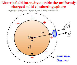 The direction of electric field intensity on the Gaussian surface is radially outward which is in the direction of the area vector of the Gaussian surface. i.e. ($\theta=0^{\circ}$). Here $\overrightarrow {dA}$ is a small area around point $P$ so the small electric flux $d\phi_{E}$ will pass through this small area $\overrightarrow {dA}$. so this flux can be found by applying Gauss's law in question given below:
$ d\phi_{E}= \overrightarrow {E}\cdot \overrightarrow{dA}$
$ d\phi_{E}= E\:dA\: cos\: 0^{\circ} \quad \left \{\because \theta=0^{\circ} \right \}$
$ d\phi_{E}= E\:dA \quad (1) \quad \left \{\because cos\:0^{\circ}=1 \right \}$
The electric flux passes through the entire Gaussian surface, So integrate the equation $(1)$ →
$ \oint d\phi_{E}= \oint E\:dA $
$\phi_{E}=\oint E\:dA\qquad (2)$
According to Gauss's law:
$ \phi_{E}=\frac{q}{\epsilon_{0}}\qquad (3)$
From equation $(2)$ and equation $(3)$, we can write as
$ \frac{q}{\epsilon_{0}}=\oint E\:dA$
$ \frac{q}{\epsilon_{0}}= E\oint dA$
Now substitute the area of the entire Gaussian spherical is $\oint {dA}=4\pi r^{2}$ in the above equation. So the above equation can be written as:
$ \frac{q}{\epsilon_{0}}= E(4\pi r^{2})$
$ E=\frac{1}{4\pi \epsilon_{0}}\frac{q}{r^{2}}$
From the above equation, we can conclude that the behavior of the electric field at the external point due to the uniformly charged solid conducting sphere is the same as the entire charge is placed at the center, point charge
If the surface charge density is $\sigma$, Then the total charge $q$ on the surface of a solid conducting sphere is→
$ q=4\pi R^{2}\: \sigma$
Substitute this value of charge $q$ in the above equation, so we can write the equation as:
$ E=\frac{1}{4\pi \epsilon_{0}}\frac{4\pi R^{2}\: \sigma}{r^{2}}$
$ E=\frac{\sigma}{\epsilon_{0}}\frac{R^{2}}{r^{2}}$
This equation describes the electric field intensity at the external point of the solid conducting sphere.
2.) Electric field intensity on the surface of the solid conducting sphere:
 If point $P$ is placed on the surface of the solid conducting sphere i.e. ($r=R$). so electric field intensity on the surface of the solid conducting sphere can be found by putting $r=R$ in the formula of electric field intensity at the external point of the solid conducting sphere:
$ E=\frac{1}{4\pi \epsilon_{0}}\frac{q}{R^{2}}$
$ E=\frac{\sigma}{\epsilon_{0}}$
3.) Electric field intensity inside the solid conducting sphere:
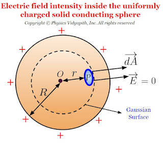 If point $P$ is placed inside the solid conducting sphere then electric field intensity will be zero because the charge is distributed uniformly on the surface of the solid sphere and there will not be any charge on the Gaussian surface. So the electric flux will be zero inside the solid sphere. i.e.
$ \phi_{E}=\oint E\:dA$
$ 0=E\oint dA \qquad\quad \left \{ \because \phi_{E}=0 \right \}$
$ E=0$
Electric field intensity distribution with distance for Conducting Solid Sphere:
 Electric field intensity distribution with distance shows that the electric field is maximum on the surface of the sphere and zero inside the sphere. Electric field intensity distribution outside the sphere reduces with the distance according to $E=\frac{1}{r^{2}}$.
B.) Electric field intensity at different points in the field due to the uniformly charged solid non-conducting sphere:
Let us consider, A solid non-conducting sphere of radius R in which $+q$ charge is distributed uniformly in the entire volume of the sphere. So electric field intensity at a different point due to the solid charged non-conducting sphere:
1.) Electric field intensity outside the solid non-conducting sphere:
Let us consider, An external point $P$ which is at a distance $r$ from the center point $O$ of the sphere. The electric flux is radially outward in the sphere. So the direction of the electric field vector and the small area vector will be in the same direction i.e. ($\theta =0^{\circ}$). Here $\overrightarrow {dA}$ is a small area, the small amount of electric flux will pass through this area i.e. →
$ d\phi_{E}= \overrightarrow {E}\cdot \overrightarrow{dA}$
$ d\phi_{E}= E\:dA\: cos\: 0^{\circ} \quad \left \{\because \theta=0^{\circ} \right \}$
$ d\phi_{E}= E\:dA \qquad (1) \quad \left \{\because cos\:0^{\circ}=1 \right \}$
 The electric flux passes through the entire Gaussian surface, So integrate the equation $(1)$ →
$ \phi_{E}=\oint E\:dA\qquad (2)$
According to Gauss's law:
$ \phi_{E}=\frac{q}{\epsilon_{0}}\qquad (3)$
From equation (1) and equation (2), we can write as
$ \frac{q}{\epsilon_{0}}=\oint E\:dA$
$ \frac{q}{\epsilon_{0}}= E\oint dA$
Now substitute the area of the entire Gaussian spherical surface is $\oint {dA}=4\pi r^{2}$ in the above equation. So the above equation can be written as:
$ \frac{q}{\epsilon_{0}}= E(4\pi r^{2})$
$ E=\frac{1}{4\pi \epsilon_{0}}\frac{q}{r^{2}}$
From the above equation, we can conclude that the behavior of the electric field at the external point due to the uniformly charged solid non-conducting sphere is the same as the point charge i.e. like the entire charge is placed at the center.
Since the sphere is a non-conductor so the charge is distributed in the entire volume of the sphere. So charge distribution can calculate by volume charge density →
$q=\frac{4}{3} \pi R^{3} \rho $
Substitute this value of charge $q$ in the above equation, so we can write the equation as:
$ E=\frac{1}{4\pi \epsilon_{0}}\frac{4\pi R^{3}\: \rho}{3r^{2}}$
$ E=\frac{\rho}{\epsilon_{0}}\frac{R^{3}}{3r^{2}}$
This equation describes the electric field intensity at the external point of the solid non-conducting sphere.
2.) Electric field intensity on the surface of the solid non-conducting sphere:
 If point $P$ is placed on the surface of a solid non-conducting sphere i.e. ($r=R$). so electric field intensity on the surface of a solid non-conducting sphere can be found by putting $r=R$ in the formula of electric field intensity at the external point of the solid non-conducting sphere:
$ E=\frac{1}{4\pi \epsilon_{0}}\frac{q}{R^{2}}$
$ E=\frac{\rho R}{3\epsilon_{0}}$
3.) Electric field intensity inside the solid non-conducting sphere:
 If point $P$ is placed inside the sphere and the distance from the origin $O$ is $r$, the electric flux which is passing through the Gaussian surface
$ \phi_{E}= E.4\pi r^{2}$
Where $\phi_{E}=\frac{q'}{\epsilon_{0}}$
$ \frac{q'}{\epsilon_{0}}=E.4\pi r^{2}$
Where $q'$ is part of charge $q$ which is enclosed with Gaussian Surface
$ E=\frac{1}{4 \pi \epsilon_{0}} \frac{q'}{r^{2}} \qquad \qquad (4)$
The charge is distributed uniformly in the entire volume of the sphere so volume charge density $\rho$ will be the same as the entire solid sphere i.e.
$ \rho=\frac{q}{\frac{4}{3}\pi R^{3}}=\frac{q'}{\frac{4}{3}\pi r^{3}}$
$ \frac{q}{\frac{4}{3}\pi R^{3}}=\frac{q'}{\frac{4}{3}\pi r^{3}}$
$ q'=q\frac{r^{3}}{R^{3}}$
$ q'=q\left (\frac{r}{R} \right)^{3}$
Put the value of $q'$ in equation $(4)$, so
$ E=\frac{1}{4\pi \epsilon_{0}}\frac{q}{r^{2}}\left(\frac{r}{R} \right)^{3}$
$ E=\frac{1}{4\pi \epsilon_{0}}\frac{qr}{R^{3}}$
Where $q=\frac{4}{3} \pi R^{3} \rho $. So above equation can be written as:
$ E=\frac{1}{4\pi \epsilon_{0}}\frac{\frac{4}{3} \pi R^{3} \rho r}{R^{3}}$
$E=\frac{ \rho r}{3 \epsilon_{0}}$
Electric field intensity distribution with distance for non-conducting Solid Sphere:
 Electric field intensity distribution with distance shows that the electric field is maximum on the surface of the sphere and zero at the center of the sphere. Electric field intensity distribution outside the sphere reduces with the distance according to $E=\frac{1}{r^{2}}$.
2.) Electric field intensity on the surface of the solid conducting sphere
3.) Electric field intensity inside the solid conducting sphere
2.) Draw a spherical surface of radius r which passes through point $P$. This hypothetical surface is known as the Gaussian surface.
3.) Now take a small area $\overrightarrow {dA} $ around point $P$ on the Gaussian surface to find the electric flux passing through it.
4.) Now find the direction between the electric field vector and a small area vector.


- Electric field intensity outside the solid non-conducting sphere
- Electric field intensity on the surface of the solid non-conducting sphere
- Electric field intensity inside the non-solid conducting sphere


Derivation of Planck's Radiation Law
Derivation:
Let $ N$ be the total number of Planck’s oscillators and $E$ be their total energy, then the
average energy per Planck’s oscillator is
$ \overline{E}=\frac{E_{N}}{N}
\qquad (1)$
Let there be $ N_{0}, N_{1} ,N_{2}
,N_{3},---N_{n}$ oscillator having energy $ E_{0}, E_{1}, E_{2}, -- E_{n}$
respectively.
According to Maxwell’s distribution, the number of oscillators in the $ n^{th}$ energy
state is related to the number of oscillators in the ground state by
$ N_{n}=N _{0} e^{\tfrac{-nh\nu }{kt} }\qquad (2)$
Where
$ n$ is a positive integer. So put $ n= 1,2,3,…….$. The above equation can be
written for different energy states. i.e.
$ N_{1}=
N _{0} e^{\tfrac{-h\nu }{kt} }$
$ N_{2}=
N _{0} e^{\tfrac{-2h\nu }{kt} }$
$ N_{3}=
N _{0} e^{\tfrac{-3h\nu }{kt} }$
$.............$
$.............$
So, the total number of Planck’s Oscillators –
$ N= N _{0} +N_{1}+N_{2}+N_{3}+.... N_{n}$
Let $ x = e^{\frac{-h\nu }{kt}} \qquad (4) $
Then $ N = N_{0}[1+x+x^{2}+x^{3}+...+ x^{n}]$
$ N = \frac{N_{0}}{1-x} \qquad(5)$ [ from Binomial theorem]
Now the total energy of oscillators –
From equation $(4)$ put $ x = e^{\tfrac{-h\nu }{kt}}$ in above equation. i.e
$ E_{N } = N_{0}h\nu (x+2x^{2}+3x^{3}+...+nx^{n}) $
$ E_{N } = N_{0}h\nu x(1+2x+3x^{2}+....)$
$ E_{N } = \frac{N_{0}h\nu x}{(1-x)^{2}} \qquad(6)$ (from Bionomical theorem)
Now substituting the value of $N$ from equation $ (5)$ and $ E_{n}$ from equation
$ (6)$ in equation $ (1)$ –
$ \overline{E}= \frac{\frac{N_{0}h\nu x}{(1-x)^{2}}}{\frac{N_{0}}{(1-x)}}$
$ \overline{E}= \frac{h\nu }{(\frac{1}{x}-1)}$
$ \overline{E}= \frac{h\nu }{e^{\tfrac{h\nu }{kt}}-1} \qquad(7)$
The
number of oscillators per unit volume in wavelength range to $ ( \lambda + d\lambda )$ is $\frac{8\pi }{\lambda ^{4}} d\lambda$.
The energy per unit volume $ (E_{\lambda }d\lambda )$ in the wavelength range to $( \lambda
+d\lambda ) $ is –
$ E_{\lambda}d\lambda = \frac{8\pi }{\lambda ^{4}}d\lambda \overline{E} \qquad(8)$
From equation $ (7)$ and $ (8)$ –
$ E_{\lambda}d\lambda = \frac{8\pi }{\lambda ^{4}}d\lambda \frac{h\nu }{(e^{\tfrac{h\nu}{kt}}-1)}$
$ E_{\lambda}d\lambda = \frac{8\pi hc}{\lambda ^{5}} \frac{d\lambda}{(e^{\tfrac{hc}{\lambda kt}}-1)}$
The above equation describes Planck’s radiation law and this law was able to thoroughly explain the black body radiation spectrum.
Wien’s Displacement law from Planck’s Radiation Law:
Planck’s radiation law gives the energy in wavelength region $ \lambda to \lambda +d\lambda $ as –
$ E_{\lambda}d \lambda = \frac{8\pi hc}{\lambda ^{5}}(\frac{1}{e^{\tfrac{hc}{\lambda kt}}-1})d\lambda \qquad(1)$
For shorter wavelength $ \lambda T$ will be small and hence
$ e^{\tfrac{hc}{\lambda kt}}> > 1$
Hence, for a small value of $\lambda T$ Planck’s formula reduces to -
$ E_{\lambda}d \lambda = \frac{8\pi hc}{\lambda ^{5}}(\frac{1}{e^{\tfrac{hc}{\lambda kt}}})
d\lambda$
$ E_{\lambda}d\lambda = \frac{8\pi hc}{\lambda ^{5}}e^{\tfrac{-hc}{\lambda kt}}d\lambda$
$E_{\lambda}d\lambda = A \lambda ^{-5} e^{\tfrac{-hc}{\lambda kt}}d\lambda$
Where $ A = 8\pi hc$
The above equation is Wien’s law of energy distribution verified by Planck
radiation law.
Rayleigh-Jeans law from Planck’s Radiation Law:
According to Planck’s radiation law –
$ E_{\lambda}.d\lambda = \frac{8\pi hc}{\lambda ^{5}}\frac{1 }{e^{\tfrac{hc}{\lambda
kt}}-1}.d\lambda$
For longer wavelength $ e^{\frac{hc}{\lambda kt}}$ is small and can be expanded as-
$ e^{\tfrac{hc}{\lambda kt}} = 1+\frac{hc}{\lambda kt}+\frac{1}{2!}(\frac{hc}{\lambda kt})^{2}+....$
Neglecting the higher-order term –
$ e^{\tfrac{hc}{\lambda kt}} = 1+\frac{hc}{\lambda kt}$
Hence for longer wavelength, Planck’s formula reduces to –
$ E_{\lambda}.d\lambda = \frac{8\pi kt}{\lambda ^{5}}[\frac{1}{1+\frac{hc}{\lambda kt}-1}]$
$ E_{\lambda}.d\lambda = \frac{8\pi kt}{\lambda ^{4}}.d\lambda$
This is Rayleigh Jean’s law verified by Planck Radiation Law.
$ N= N _{0} + N_{0} e^{\tfrac{-h\nu }{kt}}+ N_{0} e^{\tfrac{-2h\nu
}{kt}}+...+ N_{0}e^{\tfrac{-nh\nu }{kt}}$
$ N= N _{0}[1+e^{\tfrac{-h\nu }{kt}}+e^{\tfrac{-2h\nu }{kt}}+.... e^{\tfrac{-nh\nu }{kt}}] \qquad(3)$
$ E_{N} = E_{0}N_{0}+ E_{1}N_{1}+ E_{2}N_{2}+...+ E_{n}N_{n}$
$ E_{N } = 0.N_{0}+ h\nu N_{0} e^{\tfrac{-h\nu }{kt}}+...+nh\nu N_{0} e^{\tfrac{-nh\nu }{kt}}$
$ E_{N } = N_{0}h\nu (e^{\tfrac{-h\nu }{kt}}+2e^{\tfrac{-2h\nu }{kt}}+...+ ne^{\tfrac{-nh\nu }{kt}})$
Orthogonality of the wave functions of a particle in one dimension box or infinite potential well
Description of Orthogonality of the wave functions of a particle in one dimension box or infinite potential well:
Let $\psi_{n}(x)$ and $\psi_{m}(x)$ be the normalized wave functions of a particle in the interval $(0, L)$ corresponding to the different energy level $E_{n}$ and $E_{m}$ respectively. These wave functions are:
$\psi_{n}(x)= \sqrt{\frac{2}{L}} sin \frac{n \pi x}{L}$
$\psi_{m}(x)= \sqrt{\frac{2}{L}} sin \frac{m \pi x}{L}$
Where $m$ and $n$ are integers.
In this function are real. Therefore
$\psi_{n}^{*}(x) = \psi_{n}(x)$
$\psi_{m}^{*}(x) = \psi_{m}(x)$
Where $m=n$,
$\int_{0}^{L} \psi_{n}^{*}(x) \psi_{m}^{*}(x) dx =0$
Hence, The function is mutually orthogonal in the interval $(0, L)$. These functions $\psi_{n}(x)$ and $\psi_{m}(x)$ are also normalized in this interval. The wave function, which is normalized and mutually orthogonal in an interval is said to form an orthogonal set in this interval. Since the wave function are zero outside the interval $(0, L)$, they are also orthogonal wave function in the whole range of $x$ axis in the interval $(-\infty, +\infty)$.
$\int_{0}^{L} \psi_{n}^{*}(x) \psi_{m}^{*}(x) dx = \frac{2}{L} \int_{0}^{L} sin \frac{m \pi x}{L} . sin \frac{n \pi x}{L} dx$
$\int_{0}^{L} \psi_{n}^{*}(x) \psi_{m}^{*}(x) dx =\frac{1}{L} \int_{0}^{L} \left[ cos \left\{ \frac{(m-n) \pi x}{L} \right\} - cos \left\{ \frac{(m+n) \pi x}{L} \right\} \right] dx $
$\int_{0}^{L} \psi_{n}^{*}(x) \psi_{m}^{*}(x) dx =\frac{1}{L} \left[ \frac{L}{\pi(m-n)} sin \left\{ \frac{(m-n) \pi x}{L} \right\} - \frac{L}{\pi(m+n)} sin \left\{ \frac{(m+n) \pi x}{L} \right\} \right]_{0}^{L} $
$\int_{0}^{L} \psi_{n}^{*}(x) \psi_{m}^{*}(x) dx =\frac{1}{L} \left[ \frac{L}{\pi(m-n)} sin \left\{ \frac{(m-n) \pi x}{L} \right\} - \frac{L}{\pi(m+n)} sin \left\{ \frac{(m+n) \pi x}{L} \right\} \right]_{0}^{L} $
The electric potential at different points (like on the axis, equatorial, and at any other point) of the electric dipole
Electric Potential due to an Electric Dipole:
The electric potential due to an electric dipole can be measured at different points:
1.) The electric potential on the axis of the electric dipole
2.) The electric potential on the equatorial line of the electric dipole
3.) The electric potential at any point of the electric dipole
1. The electric potential on the axis of the electric dipole:
Let us consider an electric dipole AB made up of two charges of -q and +q coulomb placed in a vacuum or air at a very small distance of $l$. Let a point $P$ be on the axis of an electric dipole and placed at a distance $r$ from the center point $O$ of the electric dipole. Now put the test charged particle $q_{0}$ at point $P$ for the measurement of the electric potential due to the dipole's charges.
 So Electric potential at point $P$ due $+q$ charge of electric dipole→
$ V_{+q}=\frac{1}{4\pi \epsilon_{0}} \frac{q}{r-\frac{l}{2}}$
The electric potential at point $P$ due $-q$ charge of electric dipole→
$ V_{-q}=-\frac{1}{4\pi \epsilon_{0}} \frac{q}{r+\frac{l}{2}}$
Electric potential is a scalar quantity. Hence, the resultant potential $V$ at the point $P$ will be the algebraic sum of the potential $V_{+q}$ and $V_{-q}$. i.e. →
$ V=V_{+q}+V_{-q}$
Now substitute the value of $V_{+q}$ and $V_{-q}$ in the above equation →
$ V= \frac{1}{4\pi \epsilon_{0}} \frac{q}{r-\frac{l}{2}} -\frac{1}{4\pi \epsilon_{0}} \frac{q}{r+\frac{l}{2}}$
$ V= \frac{1}{4\pi \epsilon_{0}} \left[ \frac{q}{r-\frac{l}{2}} - \frac{q}{r+\frac{l}{2}} \right]$
$ V= \frac{q}{4\pi \epsilon_{0}} \left[ \frac{1}{r-\frac{l}{2}} - \frac{1}{r+\frac{l}{2}} \right]$
$ V= \frac{q}{4\pi \epsilon_{0}} \left[ \frac{ \left( r+\frac{l}{2} \right)-\left (r-\frac{l}{2} \right)}{r^{2}-\frac{l^{2}}{4}} \right]$
$ V= \frac{1}{4\pi \epsilon_{0}} \left[ \frac{ql}{r^{2}-\frac{l^{2}}{4}} \right]$
$ V= \frac{1}{4\pi \epsilon_{0}} \left[ \frac{p}{r^{2}-\frac{l^{2}}{4}} \right] \qquad \left( \because p=ql\right)$
If $r$ is much larger than $l$. So $\frac{l^{2}}{4}$ can be neglected in comparison to $r^{2}$. Therefore, the electric potential at the point $P$ due to the electric dipole is →
$ V= \frac{1}{4\pi \epsilon_{0}} \left[ \frac{p}{r^{2}} \right] $
2. The electric potential on the equatorial line of the electric dipole:
Let us consider an electric dipole AB made up of two charges of $+q$ and $-q$ coulomb placed in a vacuum or air at a very small distance of $l$. Let a point $P$ be on the equatorial line of an electric dipole and place it at a distance $r$ from the center point $O$ of the electric dipole. Now put the test charged particle $q_{0}$ at point $P$ for the measurement of the electric potential due to the dipole's charges.
 So Electric potential at point $P$ due $+q$ charge of electric dipole→
$ V_{+q}=\frac{1}{4\pi \epsilon_{0}} \frac{q}{BP}$
$ V_{+q}=\frac{1}{4\pi \epsilon_{0}} \frac{q}{\sqrt{r^{2}+\frac{l^{2}}{4}}}$
The electric potential at point $P$ due $-q$ charge of electric dipole→
$ V_{-q}=-\frac{1}{4\pi \epsilon_{0}} \frac{q}{AP}$
$ V_{-q}=-\frac{1}{4\pi \epsilon_{0}} \frac{q}{\sqrt{r^{2}+\frac{l^{2}}{4}}}$
$\therefore$ The resultant potential at point $P$ is
$ V=V_{+q}+V_{-q}$
$ V=\frac{1}{4\pi \epsilon_{0}} \frac{q}{\sqrt{r^{2}+\frac{l^{2}}{4}}}-\frac{1}{4\pi \epsilon_{0}} \frac{q}{\sqrt{r^{2}+\frac{l^{2}}{4}}} $
$V=0 $
Thus, the electric potential is zero on the equatorial line of a dipole (but the intensity is not zero). So, no work is done in moving a charge along this line.
3. The electric potential at any point of the electric dipole:
Let us consider an electric dipole $AB$ of length $l$ consisting of the charge $+q$ and $-q$. Let's take a point $P$ in general, and its distance is $r$ from the center point $O$ of the electric dipole AB.
Let the distance of point $P$ from the point $A$ and Point $B$ of the dipole is $PB=r_{1}$ and $PA=r_{2}$ respectively.
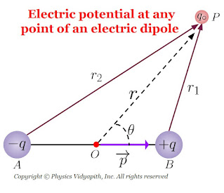 So, the electric potential at point $P$ due to the $+q$ charge of the electric dipole is →
$ V_{+q}=\frac{1}{4\pi \epsilon_{0}} \frac{q}{r_{1}}$
$ V_{-q}=-\frac{1}{4\pi \epsilon_{0}} \frac{q}{r_{2}}$
The resultant potential at point $P$ is the algebraic sum of the potential due to charges $+q$ and $-q$ of the dipole. That is
$ V=V_{+q}+V_{-q}$
$ V=\frac{1}{4\pi \epsilon_{0}} \frac{q}{r_{1}}-\frac{1}{4\pi \epsilon_{0}} \frac{q}{r_{2}}$
$ V=\frac{1}{4\pi \epsilon_{0}} \left(\frac{q}{r_{1}}-\frac{q}{r_{2}} \right) \qquad(1)$
Now simplify the above equation by applying the Geometry from the above figure. i.e. From the figure, Acute angle $\angle POB$, we can write as,
$ r^{2}_{1}=r^{2}+\frac{l^{2}}{4}-rlcos\theta \qquad(2)$
Similarly for displacement $\overrightarrow{r_{2}}$
$ r^{2}_{2}=r^{2}+\frac{l^{2}}{4}-rlcos \left(\pi - \theta \right)$
$ r^{2}_{2}=r^{2}+\frac{l^{2}}{4}+rlcos \theta \qquad(3)$
The equation $(2)$ may be expressed as →
$ r^{2}_{1}=r^{2} \left[1+ \frac{l^{2}}{4r^{2}}-\frac{l}{r}cos\theta \right] $
Taking distance $r$ much greater than the length of dipole (i.e. r>>l), so we may retain only the first order term in $\frac{l}{r}$,
$ \therefore r^{2}_{1}=r^{2} \left[1- \frac{l}{r}cos\theta \right]$
$ r_{1}=r \left[1- \frac{l}{r}cos\theta \right]^{\frac{1}{2}}$
$ \frac {1}{r_{1}}=\frac{1}{r} \left[1- \frac{l}{r}cos\theta \right]^{-\frac{1}{2}}$
Now, applying the binomial theorem to the above equation. So we get
$ \frac {1}{r_{1}}=\frac{1}{r} \left[1+ \frac{l}{2r}cos\theta \right]$
Similarly,
$ \frac {1}{r_{2}}=\frac{1}{r} \left[1- \frac{l}{2r}cos\theta \right]$
Substituting these values in equation $(1)$, we get
$ V=\frac{1}{4\pi\epsilon_{0}} \left[ \frac{q}{r} \left(1+ \frac{l}{2r}cos\theta \right)-\frac{q}{r} \left(1- \frac{l}{2r}cos\theta \right)
\right]$
$ V=\frac{1}{4\pi\epsilon_{0}}\frac{q}{r} \left[ \left(1+ \frac{l}{2r}cos\theta \right)- \left(1- \frac{l}{2r}cos\theta \right) \right]$
$ V=\frac{1}{4\pi\epsilon_{0}}\frac{q}{r} \left[ \left(1+ \frac{l}{2r}cos\theta \right)- \left(1- \frac{l}{2r}cos\theta \right) \right]$
$ V=\frac{1}{4\pi\epsilon_{0}}\frac{q}{r} \left[ \frac{l cos\theta}{r}\right]$
$ V=\frac{1}{4\pi\epsilon_{0}} \left[ \frac{ql cos\theta}{r^{2}}\right]$
But $q\times l=p$ (dipole moment)
$ V=\frac{1}{4\pi\epsilon_{0}} \left[ \frac{p cos\theta}{r^{2}}\right]$
The vector form of the above equation can be written as →
$ V=\frac{1}{4\pi\epsilon_{0}} \left[ \frac{\overrightarrow{p} \cdot \overrightarrow{r} }{r^{3}}\right]$
The above two equations hold only under the approximation that the distance of the observation point $P$ is much greater than the size of the dipole.
Special Case:
Now comparing this result with the potential due to a point-charge, we see that:
2.) The electric potential on the equatorial line of the electric dipole
3.) The electric potential at any point of the electric dipole


- At axial points $\theta=0^{\circ}$,
then $cos\theta= cos 0^{\circ}=1$,Therefore, $ V=\frac{1}{4\pi\epsilon_{0}} \frac{p}{r^{2}}$
- At equatorial points $\theta=90^{\circ}$,
then $cos\theta= cos 90^{\circ}=0$,Therefore,$ \quad V=0$
- In a fixed direction, that is, fixed $\theta$, $V\propto \frac{1}{r^{2}}$. here rather than $V \propto \frac{1}{r}$;
- Even for a fixed distance $r$, there is now a dependence on direction, that is, on $\theta$.
Electric field intensity due to uniformly charged plane sheet and parallel sheet
Electric field intensity due to a uniformly charged infinite plane thin sheet:
Let us consider, A plane charged sheet (It is a thin sheet so it will have
surface charge distribution whether it is a conducting or nonconducting
sheet) whose surface charge density is $\sigma$. From symmetry, Electric
field intensity is perpendicular to the plane everywhere and the field
intensity must have the same magnitude on both sides of the sheet. Let point
$P_{1}$ and $P_{2}$ be the two-point on the opposite side of the sheet.
To use Gaussian law, we construct a cylindrical Gaussian surface of
cross-section area $\overrightarrow{dA}$, which cuts the sheet, with points
$P_{1}$ and $P_{2}$. The electric field $\overrightarrow{E}$ is normal to
end faces and is away from the plane. Electric field $\overrightarrow{E}$ is
parallel to cross-section area $\overrightarrow{dA}$. Therefore the curved
cylindrical surface does not contribute to the flux i.e. $\oint
\overrightarrow{E} \cdot \overrightarrow{dA}=0$.Hence the total flux is
equal to the sum of the contribution from the two end faces. Thus, we get
$ \phi_{E}=\int_{A} \overrightarrow{E} \cdot
\overrightarrow{dA}+\int_{A} \overrightarrow{E} \cdot \overrightarrow{dA}$
$ \phi_{E}= \int_{A} E \: dA \:cos 0^{\circ} +\int_{A} E \: dA \:cos
0^{\circ} $
Here the direction of $\overrightarrow{E}$ and $\overrightarrow{dA}$ is same. So the angle will be $\theta = 0^{\circ}$.
$ \phi_{E}= \int_{A} E \: dA +\int_{A} E \: dA $
$ \phi_{E}= \int_{A} 2E \: dA $
$ \phi_{E}= 2E \int_{A} \: dA $
$ \phi_{E}= 2E\:A $
$ \frac{q}{\epsilon_{0}}=2E\:A \qquad \left \{\because
\phi_{E}=\frac{q}{\epsilon_{0}} \right \}$
$ E=\frac{q}{2\epsilon_{0} A}$
$\because q=\sigma A $, So the above equation can be written as:
$ E=\frac{\sigma A}{2\epsilon_{0} A} $
$ E=\frac{\sigma}{2\epsilon_{0}} $
Electric field intensity due to the uniformly charged infinite conducting
plane thick sheet or Plate:
Let us consider that a large positively charged plane sheet having a finite
thickness is placed in the vacuum or air. Since it is a conducting plate so the
charge will be distributed uniformly on the surface of the plate. Let
$\sigma$ be the surface charge density of the charge
Let's take a point $P$ close to the plate at which electric field intensity
has to determine. Since there is no charge inside the conducting plate, this
conducting plate can be assumed as equivalent to two plane sheets of charge
i.e sheet 1 and sheet 2.
The magnitude of the electric field intensity $\overrightarrow {E_{1}}$ at point $P$ due to sheet 1 is →
$ E_{1}=\frac{\sigma}{2\epsilon_{0}}$ (away from sheet 1)
The magnitude of the electric field intensity $\overrightarrow {E_{2}}$ at
point $P$ due to sheet 2 is →
$ E_{2}=\frac{\sigma}{2\epsilon_{0}}$ (away from sheet 2)
Since $\overrightarrow {E_{1}}$ and $\overrightarrow {E_{2}}$ are in the
same direction, the magnitude of resultant intensity $\overrightarrow {E}$
at point $P$ due to both the sheet is →
$ E=E_{1}+E_{2}$
$\because \quad E=\frac{\sigma}{2\epsilon_{0}}+\frac{\sigma}{2\epsilon_{0}}$
$ E=\frac{\sigma}{\epsilon_{0}} $
The resultant electric field will be away from the plate. If the plate is
negatively charged, the electric field intensity $\overrightarrow {E}$ would
be directed toward the plate.
We have obtained the above formula for a 'plane' charged conductor. In fact,
it holds for the electric field intensity 'just' outside a charged conductor
of any shape.
Electric field intensity due to two Infinite Parallel Charged Sheets:
When both sheets are positively charged:
Let us consider, Two infinite, plane, sheets of positive charge, 1 and 2 are
placed parallel to each other in the vacuum or air. Let $\sigma_{1}$ and
$\sigma_{2}$ be the surface charge densities of charge on sheet 1 and 2
respectively.
Let $\overrightarrow {E_{1}}$ and $\overrightarrow {E_{2}}$ be the electric
field intensities at any point due to sheet 1 and sheet 2 respectively.
Then,
The electric field intensity at points $P'$ →
$ E_{1}=\frac{\sigma_{1}}{2\epsilon_{0}}$ (away from sheet 1)
$ E_{2}=\frac{\sigma_{2}}{2\epsilon_{0}}$ (away from sheet 2)
Since, Electric field intensities $\overrightarrow {E_{1}}$ and
$\overrightarrow {E_{2}}$ are in the same direction, the magnitude of
resultant intensity at point $P'$ is given by →
$ E=E_{1}+E_{2}$
$ E=\frac{\sigma_{1}}{2 \epsilon_{0}}+\frac{\sigma_{2}}{2
\epsilon_{0}}$
$ E=\frac{1}{2 \epsilon_{0}} \left (\sigma_{1}+\sigma_{2} \right )$
If both sheets have equal charge densities $\sigma$ i.e.
$\sigma_{1}=\sigma_{2}=\sigma$, Then above equation can be written as:
$ E=\frac{\sigma}{ \epsilon_{0}} $
This electric field intensity would be away from both sheet 1 and sheet 2.
The electric field intensity at points $P$→
Electric field intensity at point $P$ due to sheet 1 is →
$ E_{1}=\frac{\sigma_{1}}{2\epsilon_{0}}$ (away from sheet 1)
$ E_{2}=\frac{\sigma_{2}}{2\epsilon_{0}}$ (away from sheet 2)
Now, both electric field intensities $\overrightarrow{E_{1}}$ and
$\overrightarrow{E_{2}}$ are in opposite direction. The magnitude of
resultant electric field $\overrightarrow{E}$ at point $P$ is given by
$ E= E_{1}-E_{2}$
$ E=\frac{\sigma_{1}}{2 \epsilon_{0}}-\frac{\sigma_{2}}{2
\epsilon_{0}}$
$ E=\frac{1}{2 \epsilon_{0}} \left (\sigma_{1}-\sigma_{2} \right )$
If both sheets have equal charge densities $\sigma$ i.e.
$\sigma_{1}=\sigma_{2}=\sigma$, Then above equation can be written as:
$ E=0 $
The electric field intensity at points $P''$ →
$ E_{1}=\frac{\sigma_{1}}{2\epsilon_{0}}$ (away from sheet 1)
$ E_{2}=\frac{\sigma_{2}}{2\epsilon_{0}}$ (away sheet 2)
Since, Electric field intensities $\overrightarrow {E_{1}}$ and
$\overrightarrow {E_{2}}$ are in the same direction, the magnitude of
resultant intensity at point $P''$ is given by →
$ E=E_{1}+E_{2}$
$ E=\frac{\sigma_{1}}{2 \epsilon_{0}}+\frac{\sigma_{2}}{2
\epsilon_{0}}$
$ E=\frac{1}{2 \epsilon_{0}} \left (\sigma_{1}+\sigma_{2} \right )$
If both sheets have equal charge densities $\sigma$ i.e.
$\sigma_{1}=\sigma_{2}=\sigma$, Then above equation can be written as:
$ E=\frac{\sigma}{ \epsilon_{0}} $
This electric field intensity would be away from both sheet 1 and sheet 2.
When one-sheet is positively charged and the other sheet negatively charged:
Let us consider two sheets 1 and 2 of positive and negative charge densities
$\sigma_{1}$ and $\sigma_{2}$ ($\sigma_{1} > \sigma_{2}$)
The electric field intensities at point $P'$ →
$ E_{1}=\frac{\sigma_{1}}{2\epsilon_{0}}$ (away from sheet 1)
$ E_{2}=\frac{\sigma_{2}}{2\epsilon_{0}}$ (toward from sheet 2)
The magnitude of the resultant electric field $E$
$ E=E_{1}-E_{2}$
$E= \frac{1}{2\epsilon_{0}} \left ( \sigma_{1}- \sigma_{2}\right )$
If both sheets have equal charge densities $\sigma$ i.e.
$\sigma_{1}=\sigma_{2}=\sigma$, Then above equation can be written as:
$ E=0 $
The electric field intensities at point $P$ →
$ E_{1}=\frac{\sigma_{1}}{2\epsilon_{0}}$ (away from sheet 1)
$ E_{2}=\frac{\sigma_{2}}{2\epsilon_{0}}$ (towards sheet 2)
Since, Electric field intensities $\overrightarrow {E_{1}}$ and
$\overrightarrow {E_{2}}$ are in the same direction, the magnitude of
resultant intensity at point $P$ is given by →
$ E=E_{1}+E_{2}$
$ E=\frac{\sigma_{1}}{2 \epsilon_{0}}+\frac{\sigma_{2}}{2
\epsilon_{0}}$
$ E=\frac{1}{2 \epsilon_{0}} \left (\sigma_{1}+\sigma_{2} \right )$
If both sheets have equal charge densities $\sigma$ i.e.
$\sigma_{1}=\sigma_{2}=\sigma$, Then above equation can be written as:
$ E=\frac{\sigma}{ \epsilon_{0}} $
The electric field intensities at point $P''$ →
$ E_{1}=\frac{\sigma_{1}}{2\epsilon_{0}}$ (away from sheet 1)
$ E_{2}=\frac{\sigma_{2}}{2\epsilon_{0}}$ (toward from sheet 2)
The magnitude of the resultant electric field $E$ →
$ E=E_{1}-E_{2}$
$E= \frac{1}{2\epsilon_{0}} \left ( \sigma_{1}- \sigma_{2}\right )$
If both sheets have equal charge densities $\sigma$ i.e.
$\sigma_{1}=\sigma_{2}=\sigma$, Then above equation can be written as:
$ E=0 $
From the above expression, we can conclude that the magnitude of $E$ is free
from the 'position' of the point taken in the electric field between the
sheet and outside the sheet. It is also shown that the electric field
between the sheet is uniform everywhere and independent of separation
between the sheets.
 |
| Infinite plane thin sheet |
$ \phi_{E}= \int_{A} E \: dA +\int_{A} E \: dA $
 |
| Plane Charged Plate |
The magnitude of the electric field intensity $\overrightarrow {E_{1}}$ at point $P$ due to sheet 1 is →
 |
| Likely positive charged sheet |
 |
| Unlike charged parallel Sheet |
Popular Posts
-
 Angle of Acceptance → "If incident angle of light on the core for which the incident angle on the core-cladding interface equals t...
 -
 Principle: The principle of the compound microscope is based on the magnification of an image by using two lenses. Construction: A comp...
 -
Description: Unit of Energy The SI unit of energy is the Joule (J) , named after the English physicist James Prescott Joule. 1 Joule is...
-
 Derivation→ Let us consider, The charge on a parallel-plate capacitor = $q$ The area of parallel-plate = $A$ The dis...
 -
Gaussian Surface and its Properties: The Gaussian surface is a hypothetical or imaginary closed three-dimensional surface. This surface i...
-
 A.) Electric field intensity at different points in the field due to the uniformly charged solid conducting sphere: Let us consider, A s...
 -
 Derivation→ Let us consider, a current-carrying conductor $XY$ having length $l$ in which current $i$ is flowing from $X$ to $Y$. Now,...
 -
 Population of energy level: The number of atoms per unit volume in any energy level is called the population of that energy level. The...
 -
Principle of Ruby Laser → Ruby laser is the first working laser that was invented by T.H.Maima in 1960. It is a three-level solid-stat...
-
Let a plane wavefront be incident normally on slit $S_{1}$ and $S_{2}$ of equal $e$ and separated by an opaque distance $d$.The diffracted l...

