Definition and derivation of the phase velocity and group velocity of wave

Wave:
A wave is defined as a disturbance in a medium from an equilibrium condition that propagates from one region of the medium to other regions.

When such type of wave propagates in the medium a progressive change in phase takes place from one particle to the next particle.

Propagation of Wave: Wave propagation in the medium occurs with two different kinds of velocity. i.e. phase velocity and group velocity.

1. Phase Velocity:
The velocity with which plane of constant the phase of a wave propagates through the medium at a certain frequency is called the phase velocity or wave velocity.

A plane wave traveling in the positive x-direction is represented by

$y=A \: sin \omega (t-\frac{x}{v})$

Where $ \omega $ – angular frequency

$y=A \: sin(\omega t-\frac{\omega x}{v})$

$y=A \: sin(\omega t-kt) \qquad(1)$

For plane-wave $(\omega t-kx)$ is the phase of wave motion. For the plane of constant phase (wavefront). We have

$( \omega t-kx) = constant (\phi) \qquad(2)$

Differentiate with respect to time $(t)$ of the above equation

$ \omega -k.\frac{dx}{dt}=0$

$\frac{dx}{dt}=\frac{ \omega}{k}\qquad(3)$

$V_{p}=\frac{ \omega}{k} \qquad \left [ \because V_{p}= \frac{dx}{dt} \right ]$

Where $V_{p}$ - Phase Velocity of a wave

Question- Show that the phase velocity of matter-wave always exceeds the velocity of light.

Answer- Method-I

$V_{p}=\frac{ \omega }{k}$

$V_{p}=\frac{2\pi \nu }{\frac{2\pi }{\lambda }}$

$V_{p} = \frac{2 \pi h \nu}{\frac{2 \pi h}{\lambda }}$

$V_{P} = \frac{E}{P}$

$V_{P} =\frac{mc^{2}}{mv}$

$V_{P} =\frac{c^{2}}{v}$

Method-II:

$V_{P}=\nu \lambda$

$V_{P}=\frac{mc^{2}}{h} \frac{h}{mv}$

$V_{P}=\frac{c^{2}}{v}$

Where $v$ is the velocity of matter particles.

Wave packet→
A wave packet is an envelope or packet which contains the number of plane waves having different wavelengths or wavenumbers. These numbers of waves superimpose on each other and form constructive and destructive interference over a small region of space and a resultant wave obtain. The spread of amplitude of the resultant wave with distance determines the size of the wave packet. A wave packet is also called a wave group.
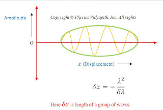
Diagram of a wave packet

Group Velocity→
The velocity of propagation of wave packet through space is known as group velocity.

Group Velocity also represents the velocity of energy flow or transmission of information in a traveling wave or wave packet. It is represented by $V_{g}$. So

$V_{g} = \frac{d\omega }{dk}$


Expression for group velocity $(V_{g})$→

Let two plane simple harmonic waves of the same amplitude and slightly different wavelength traveling simultaneously in the positive x-direction in a dispersive medium be represented by –

$y_{1} = A\: sin{(\omega t-kx)} \qquad (1)$

$y_{2}= A\:sin[(\omega +\delta \omega )t-(k+\delta k)x] \qquad (2)$

From the superposition principle the resultant displacement of waves

$y=y_{1}+y_{2}\qquad (3)$

$y=A \: sin(\omega t-kx)+ A \: sin[(\omega +\delta \omega)t-(k+\delta k)x]$

$y=A[sin(\omega t-kx)+ sin{(\omega +\delta \omega )t-(k+\delta k )x}]$

$y=2Asin(\omega t-kx)cos\frac{1}{2}(t\delta \omega –x\delta k) \qquad (4)$

This is the analytical equation for the group of waves. This equation represents the following points –
  1. The sine factors represent a carrier wave that travels with the phase velocity.

  2. The amplitude of the resultant wave is


$R=2A cos \frac{1}{2}(t \delta\omega-x \delta k) \qquad (5)$

(A) For maximum amplitude

$ cos\frac{1}{2}(\delta\omega t-x\delta k)=1 \qquad (6) $

Then the resultant amplitude of the wave packet will be

$R_{m}=2A \qquad $ {from equation $(5)$ }

Where $R_{m}$ - Resultant maximum amplitude

From equation$(6)$-

$cos\frac{1}{2}(t\delta\omega –x\delta k)=1$

$cos\frac{1}{2}(t\delta\omega –x\delta k)=cos0$

$\frac{1}{2}(t\delta\omega –x\delta k)=0$

$\frac{x}{t}=\frac{\delta\omega }{\delta k}$

$V_{g}=\frac{\delta\omega }{\delta k}$

OR

$V_{g}=\frac{d\omega}{dk}$

Thus maximum amplitude i.e. the center of the wave packet moves with velocity $\frac {d\omega}{dk}$ or group velocity.

(B) For minimum amplitude

Let a wave packet that has minimum (zero) amplitude on two successive points $x_{1}and x_{2}$. So for minimum amplitude at point $x_{1}$ –

$cos\frac{1}{2}(t.\delta \omega –x_{1}.\delta k)=0$

$cos\frac{1}{2}(t.\delta \omega –x_{1}.\delta k)=cos(2n+1)\frac{\pi }{2}$

$\frac{1}{2}(t.\delta \omega –x_{1}.\delta k)=(2n+1)\frac{\pi }{2}$

$t.\delta \omega – x_{1}.\delta k=(2n+1)\pi \qquad(1)$

Similarly minimum amplitude at the second successive point $x_{2}$-

$t\delta \omega –x_{2}.\delta k =(2n-1)\pi \qquad(2)$

Now subtract the equation $(2)$ in equation $(1)$

$(t.\delta \omega – x_{1}.\delta k) – (t.\delta \omega - x_{2}.\delta k)= (2n+1)\pi–(2n-1)\pi $

$(x_{2}-x_{1}).\delta k=2\pi$

$x_{2}-x_{1}=\frac{2\pi}{\delta k}$

$x_{2}-x_{1}=\frac{2\pi}{d(\frac{2\pi}{\lambda})} $

$\delta x=\frac{-\lambda ^{2}}{\delta  \lambda }$

Here $\delta x$ -Length of the wave packet

The above equation also can be written as-

$ dx=\frac{-\lambda^{2}}{d \lambda }$

Prove that

$V_{g}= -\lambda^{2} \frac{d\nu }{d\lambda}$

Where $\nu $ is the frequency and $\lambda $ is the wavelength.

Proof:

We know that

$V_{g}=\frac{d\omega }{dk}$

$V_{g}=\frac{d(2\pi\nu )}{d(\frac{2\pi }{\lambda })} \qquad \left( \because \omega= 2\pi \nu \: and \: k=\frac{2\pi}{\lambda } \right)$

$V_{g}=\frac{2\pi d\nu }{2\pi d( \frac{1}{ \lambda })}$

$V_{g}=-\lambda ^{2}\frac{d\nu }{d\lambda }$

Note: A moving particle cannot be equal to a single wave train. The speed of a single wave train is called the phase velocity so moving particles are equivalent to a group of waves or wave packets.

Product of phase velocity and group velocity is equal to square of speed of light

Prove that $\rightarrow$
The Product of phase velocity and group velocity is equal to the square of the speed of light i.e. $\left( V_{p}.V_{g}=c^{2} \right)$

Proof → We know that

$V_{p}=\nu \lambda \qquad(1)$

And de Broglie wavelength-

$\lambda =\frac{h }{mv}\qquad(2)$

According to Einstein's mass-energy relation-

$E=mc^{2}$

$h\nu=mc^{2}$

$\nu=\frac{mc^{2}}{h}\qquad(3)$

Now put the value of $\lambda $ and $\nu $ in equation$(1)$

$V_{p}= [\frac{mc^{2}}{h}] [\frac{h}{mv}]$

$V_{p}=\frac{C^{2}}{v}$

Since group velocity is equal to particle velocity i.e. $V_{g}=v$. So above equation can be written as

$V_{p}=\frac{C^{2}}{V_{g}}$

$V_{p}.V_{g}=C^{2}$

Note →

➢ $V_{g}=V_{p}$ for a non-dispersive medium ( in a non-dispersive medium all the waves travel with phase velocity).

➢ $V_{g}< V_{p}$ for normal dispersive medium

➢ $V_{g}> V_{p}$ for anomalous dispersive media.

Dispersive medium → The medium in which the phase velocity varies with wavelength or frequency is called a dispersive medium. In such a medium, waves of different wavelengths travel with different phase velocities.

Non-dispersive medium → The medium in which the phase velocity does not vary with wavelength or frequency is called a Non-dispersive medium.

Dispersive waves → Those waves in the medium for which phase velocity varies with wavelength or frequency are called dispersive waves.

Non-dispersive waves → Those waves in which phase velocity does not vary with wavelength are called non-dispersive waves. So phase velocity independent of wavelength.

Energy distribution spectrum of black body radiation

Description→ The energy distribution among the different wavelengths in the spectrum of black body radiation was studied by Lummer and Pringsheim in 1899. There are the following important observations of the study.
  1. The energy distribution in the radiation spectrum of the black body is not uniform. As the temperature of the body rises the intensity of radiation for each wavelength increases.

  2. At a given temperature, the intensity of radiation increases with increases in wavelength and becomes maximum at a particular wavelength with further in increases wavelength the intensity of radiation decreases.

  3. Energy distribution in the spectrum of black body
    Energy distribution in the spectrum of black body radiation
  4. The points of maximum energy shift towards the shorter wavelength as the temperature increases i.e. $\lambda _{m} \times T=constant$. It is also known as Wein’s displacement law of energy distribution.

  5. For a given temperature the total energy of radiation is represented by the area between the curve and the horizontal axis and the area increases with increases of temperature, being directly proportional to the fourth power of absolute temperatures.
    The total amount of heat radiated by a perfectly black body per unit area per unit time is directly proportional to the fourth power of its absolute temperature $(T)$.

    $E = \sigma T^{4}$

    Where $\sigma$ = Stefan constant having value $\left ({5}\cdot{67}\times{10}^{-8}Wm^{-2}K^{4}\right )$

    This is called Stefan-Boltzmann's law of energy distribution.

Derivation of torque on an electric dipole in an uniform and a non-uniform electric field

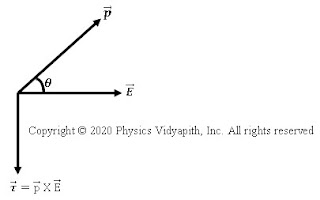
Torque on an electric dipole in a uniform electric field: Let us consider, An electric dipole AB, made up of two charges $+q$ and $-q$, is placed at a very small distance $l$ in a uniform electric field $\overrightarrow{E}$. If $\theta$ is the angle between electric field intensity $\overrightarrow{E}$ and electric dipole moment $\overrightarrow{p}$ then the magnitude of electric dipole moment →

$\overrightarrow{p}=q\times\overrightarrow{l}\qquad(1)$

Force exerted on charge $+q$ by electric field $\overrightarrow{E}$ →

$\overrightarrow{F_{+q}}=q\overrightarrow{E}\qquad(2)$

Here in the above equation(2), the direction of $\overrightarrow{F_{+q}}$ is along the direction of $\overrightarrow{E}$

Force exerted on charge $-q$ by electric field $\overrightarrow{E}$ →

$\overrightarrow{F_{-q}}= q\overrightarrow{E}\qquad(3)$

Here in the above equation(3) the direction of $\overrightarrow{F_{-q}}$ is in the opposite direction of $\overrightarrow{E}$

So, the net force of on an electric dipole→

$\overrightarrow{F}=\overrightarrow{F_{+q}} - \overrightarrow{F_{-q}}\qquad (4)$

Now substitute the value of equation $(2)$ and equation $(3)$ in above equation $(4)$. So net force→

$\overrightarrow{F}=0\qquad (5)$
Torque on Electric Dipole
Hence, the net translating force on an electric dipole in a uniform electric field is zero. But these two force is equal in magnitude, opposite in direction, and act at different point of the dipole so these force form a coupling force that exerts a torque on an electric dipole→

Torque = force x Perpendicular distance between the two forces

$\overrightarrow{\tau}=(qE).l\:sin\theta\quad\quad\quad\quad(6)$

$ \overrightarrow{\tau}=pE\:sin\theta$

$\overrightarrow{\tau}=\overrightarrow{p}\times\overrightarrow{E}$

Case(I)→ If the dipole is placed perpendicular to the electric field i.e. $\theta=90^{\circ}$, the torque acting on it will be maximum. i.e.

$ \tau_{max}=pE $

Case(II)→ If the dipole is placed parallel to the electric field i.e. $\theta=0^{\circ}$ or $\theta=180^{\circ}$, the torque acting on it will be minimum. i.e.

$ \tau_{min}=0$
Direction of torque
Direction of torque
Electric Dipole Moment:

We know that the torque

$ \overrightarrow{\tau}=pE\:sin\theta$

If $E=1$ and $\theta=90^{\circ}$ Then

$ \tau_{max} =p$

Hence Electric dipole moment is the torque acting on the dipole placed perpendicular to the direction of uniform electric field intensity.

Torque on an electric dipole in a non-uniform electric field:

In a non-uniform electric field, the $+q$ and $-q$ charges of a dipole experience different forces (not equal in magnitude and opposite in direction) at a slightly different position in the electric field, and hence a net force $\overrightarrow{F}$ act on the dipole in a non-uniform field. A net torque acts on the dipole which depends on the location of the dipole in the non-uniform field.

$\overrightarrow{\tau}=\overrightarrow{p}\times\overrightarrow{E}(\overrightarrow{r})$

Where $\overrightarrow{r}$ is the position vector of the center of the dipole.
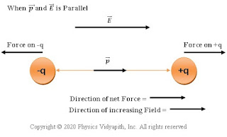
When p  and E  is Parallel
When p and E are Parallel
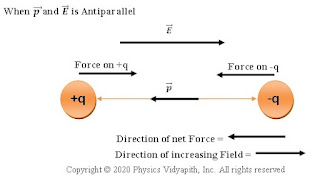
In the non-uniform field, If the direction of the dipole moment $\overrightarrow{p}$ is parallel to electric field intensity $\overrightarrow{E}$ or antiparallel to electric field intensity $\overrightarrow{E}$ the net torque on the dipole is zero because the force on charges becomes linear.
When p  and E  is antiparallel
When p and E are antiparallel
However, If $\overrightarrow{p}$ is parallel to $\overrightarrow{E}$, a net force on the dipole in the direction of increasing $\overrightarrow{E}$. When $\overrightarrow{p}$ is antiparallel to $\overrightarrow{E}$, a net force on the dipole in the direction of decreasing $\overrightarrow{E}$. As shown in the figure above.

Electric Dipole and Derivation of Electric field intensity at different points of an electric dipole

Electric Dipole:

When two equal (i.e., equal in magnitude) and opposite-charge particles are placed at a very small distance apart, the system is known as an electric dipole.

Electric Dipole Moment:

The product of magnitude of one point charged particle and the distance between the charges is called the 'electric dipole moment'. It is vector quantity and the direction of electric dipole moment is along the axis of the dipole pointing from negative charge to positive charge.
Electric Dipole System
Let us consider the two charged particles, which have equal magnitude $+q$ coulomb and $-q$ coulomb, placed at a very small distance of $l$ in a dipole, so the electric dipole moment is →

$\overrightarrow{p}=q\times \overrightarrow{l}$

Unit: $C-m$ Or $Ampere-metre-sec$

Dimension: $[ALT]$

Electric field intensity due to an Electric Dipole:

The electric field intensity due to an electric dipole can be measured at three different points:

  1. 1.) Electric field intensity at any point on the axis of an electric dipole

  2. 2.) Electric field intensity at any point on the equatorial line of an electric dipole

  3. 3.) Electric field intensity at any point on an electric dipole


1. Electric field intensity at any point on the axis of an electric dipole:

Let us consider an electric dipole $AB$ made up of two charges of $-q$ and $+q$ coulomb placed in a vacuum or air at a very small distance of $l$. Let take a point $P$ on the axis of an electric dipole and place it at a distance $r$ from the center point $O$ of the electric dipole. Now put a test charged particle $q_{0}$ at point $P$ for the measurement of the electric field intensity due to the dipole's charge.
Electric field intensity at any point on the axis of an electric dipole
So, the electric field intensity (magnitude only) at point $P$ due to a $+q$ charge of an electric dipole

$ E_{+q}=\frac{1}{4\pi\epsilon}\frac{q}{(r-\frac{l}{2})^{2}} \qquad(1)$

Electric field intensity (magnitude only) at point $P$ due $-q$ charge of electric dipole

$ E_{-q}=\frac{1}{4\pi\epsilon_{0}}\frac{q}{(r+\frac{l}{2})^{2}} \qquad(2)$

The net electric field at point $P$ due to an electric dipole

$ E=E_{+q}-E_{-q}\qquad(3)$

Subtitute the value of $E_{+q}$ and $E_{-q}$ in equation $(3)$, Then the above equation $(3)$ can also be written as follows

$E=\frac{q}{4\pi\epsilon _{0}}\left [ \frac{1}{(r-\frac{l}{2})^{2}}-\frac{1}{(r+\frac{l}{2})^{2}} \right ]$

$ E=\frac{q}{4\pi\epsilon _{0}}\left [ \frac{(r+\frac{l}{2})^{2}-(r-\frac{l}{2})^{2}}{(r+\frac{l}{2})^{2}(r-\frac{l}{2})^{2}} \right ]$

$ E=\frac{q}{4\pi\epsilon _{0}}\left [ \frac{(r^{2}+\left(\frac{l}{2}\right)^{2}+2\frac{l}{2}r-r^{2}-\left(\frac{l}{2}\right)^{2}+2\frac{l}{2}r)}{(r+\frac{l}{2})^{2}(r-\frac{l}{2})^{2}} \right ]$

$ E=\frac{q}{4\pi\epsilon _{0}}\left [ \frac{2rl}{(r^{2}-\frac{l^{2}}{4})^{2}} \right ]\qquad(4)$

Here $l \lt r $ so $\frac{l^{2}}{4} \lt \lt r^{2}$ therefore neglect the term $\frac{l^{2}}{4}$ in above equation $(4)$ so we can write above equation

$ E=\frac{q}{4\pi\epsilon _{0}}\left [ \frac{2rl}{(r^{2})^{2}} \right ]$

$E=\frac{1}{4\pi\epsilon _{0}}\left [ \frac{2p}{r^{3}} \right ]\qquad (5)$

This is the equation of electric field intensity at a point on the axis of an electric dipole.

The vector form of the above equation $(5)$ is

$\overrightarrow{E}=\frac{1}{4\pi\epsilon _{0}}\left [ \frac{2\overrightarrow{p}}{r^{3}} \right ]$

2. Electric field intensity at any point on the equatorial line of an electric dipole:

Let us consider an electric dipole $AB$ made up of two charges of $+q$ and $-q$ coulomb placed in vacuum or air at a very small distance $l$. Let a point $P$ be on the equatorial line of an electric dipole and place it at a distance $r$ from the center point $O$ of the electric dipole. Now put the test charged particle $q_{0}$ at point $P$ for the measurement of the electric field intensity due to the dipole's charge.

So, the electric field intensity (magnitude only) at point $P$ due to a $+q$ charge of an electric dipole
Electric Field Intensity on the equatorial line of dipole
$E_{+q}=\frac{1}{4\pi\epsilon_{0}}\left [\frac{q}{\left\{r^{2}+\left(\frac{l}{2}\right)^{2}\right\}} \right ] \qquad(1)$

Electric field intensity (magnitude only) at point $P$ due to $-q$ charge of electric dipole

$E_{-q}=\frac{1}{4\pi\epsilon_{0}}\left [\frac{q}{\left\{r^{2}+\left(\frac{l}{2}\right)^{2}\right\}} \right ] \qquad(2)$

The net electric field at point $P$ due to an electric dipole

$E=E_{+q}\:cos\theta + E_{-q}\: cos\theta \qquad(3)$

Put the value of $E_{+q}$ and $E_{-q}$ in the above equation $(3)$, So equation $(3)$ can also be written as follows

$E=2\left [ \frac{q}{4\pi\epsilon_{0} }\frac{1}{\left\{r^{2}+\left(\frac{l}{2}\right)^{2}\right\}} \right ]cos\theta \qquad (4)$

From figure, In $\Delta \: POB$,

$cos\:\theta=\frac{l}{\sqrt{\left\{r^{2}+\left(\frac{l}{2}\right)^{2}\right\}}}$

Put the value of $cos\theta$ in equation $(4)$, so equation $(4)$ can also be written as follows

$E=\frac{1}{4\pi\epsilon_{0}}\left [ \frac{q\times l}{\left\{r^{2}+\left(\frac{l}{2}\right)^{2}\right\}^{3/2}} \right ] \qquad (5)$

Here $l \lt r$ so $\frac{l^{2}}{4} \lt \lt r^{2}$ so neglect the term $\frac{l^{2}}{4}$ in above equation $(5)$ so we can write above equation

$ E=\frac{1}{4\pi\epsilon_{0}}\left [ \frac{q\times l}{r^{3}} \right ] \qquad (6)$

$E=\frac{1}{4\pi\epsilon_{0}} \frac{p}{r^{3}} \qquad (7)$

This is the equation of electric field intensity at a point on the equatorial line of an electric dipole.

The vector form of the above equation $(7)$ is

$\overrightarrow{E}=\frac{1}{4\pi\epsilon_{0}} \frac{\overrightarrow{p}}{r^{3}}$

3. Electric field intensity at any point of an electric dipole:

Let us consider an electric dipole $AB$ of length $l$ consisting of the charge $+q$ and $-q$. Let's take a point $P$ in general, and denote its position vector by $\overrightarrow{r}$ from the center point $O$ of the electric dipole AB to point $P$.
Electric field intensity at any point of an electric dipole
The electric dipole moment is a vector quantity that has a direction from $-q$ charge to $+q$ charge. So the electric dipole moment's direction is resolved into two components, one component $ pcosθ$ is along the vector position $\overrightarrow{r}$, and the other component $psinθ$ is normal to vector position $\overrightarrow{r}$. So

Electric field intensity due to dipole moment of component $p\:cos\theta$ {Electric field along the Axial Line }

$ \overrightarrow{E_{\parallel }}=\frac{1}{4\pi\epsilon_{0}} \frac{2pcos\theta}{r^{3}} \qquad(1)$

Electric field intensity due to dipole moment of component $p\:sin\theta$ {Electric field along the Equatorial Line}

$ \overrightarrow{E_{\perp}}=\frac{1}{4\pi\epsilon_{0}} \frac{psin\theta}{r^{3}} \qquad(2)$

The resultant electric field vector $E$ at point $P$

$ \overrightarrow{E}=\sqrt{E_{\perp}^{2}+E_{\parallel}^{2}+2 E_{\perp}E_{\parallel}cos90^{\circ}}$

From figure, The angle between $E_{\perp}$ and $E_{\parallel}$ is $90^{\circ}$. So

$\overrightarrow{E}=\sqrt{E_{\perp}^{2}+E_{\parallel}^{2} }\qquad (3)$

Now substitute the value of equation $(1)$ and equation $(2)$ in equation $(3)$. Then

$ \overrightarrow{E}=\frac{1}{4\pi\epsilon_{0}}\frac{p}{r^{3}}\sqrt{(sin^{2}\theta+4cos^{2}\theta)}$

$ \overrightarrow{E}=\frac{1}{4\pi\epsilon_{0}}\frac{p}{r^{3}}\sqrt{(1+3cos^{2}\theta)}$

This is the equation of electric field intensity at any point due to an electric dipole.

The direction of the resultant electric field intensity vector $\overrightarrow{E}$ from the axial line is

$tan\alpha =\frac{\overrightarrow{E}_{\perp }}{\overrightarrow{E_{\parallel }}} \qquad(4)$

Put the value of $\overrightarrow{E_{\perp}}$ and $\overrightarrow{E_{\parallel}}$ in equation (4). we get

$tan\alpha =\frac{sin\theta}{2cos\theta}$

$tan\alpha =\frac{1}{2}tan\theta$

Here $\alpha$ is the angle between the resultant electric field intensity $\overrightarrow{E}$ and the axial line.

Definition and Expression of escape velocity of an object on the planet

Definition of Escape Velocity:

The minimum velocity, by which an object is thrown vertically in an upward direction and that object goes out from the gravitation field of the planet and does not come back, is called the escape velocity.

Deduction Escape Velocity Expression:

Let us consider the following:

The mass of the planet =$M$
The radius of the planet = $R$
The mass of the object = $m$
An object thrown vertically upward with Escape Velocity
The gravitational force on an object at position $P$ which is a distance $x$ from the surface of the planet

$F=G\frac{M m}{x^{2}} \qquad(1)$

The work done by the force to move the object a very small distance $dx$ from position $A$ to $B$

$W=F.dx$

$dw=G\frac{M m}{x^{2}}dx$

The total work done to move the object from the surface of the planet to infinity

$\int^{W}_{0}dw= \int^{\infty}_{R}G\frac{M m}{x^{2}}dx$

$\left[ w \right]^{W}_{0}=G M m \int^{\infty}_{R} \frac{dx}{x^{2}}$

On solving the above equation

$W=GM m \int^{\infty}_{R} \frac{dx}{x^{2}}$

$W=GM m \left[ -\frac{1}{x} \right]^{\infty}_{R}$

$W=GM m \left[ -\frac{1}{\infty} + \frac{1}{R} \right]$

$W=GM m \left[\frac{1}{R} \right]$

$W=\frac{G M m}{R}$

The above work done is given to the object in the form of kinetic energy to projectile from the surface of the planet to infinity. i.e.

$\frac{1}{2} m v^{2}_{e}= \frac{G M m}{R} $

Where $v_{e}$ is the escape velocity of the object.

$v^{2}_{e} = \frac{2G M m}{R}$

$v_{e} = \sqrt{\frac{2G M}{R}} \qquad(2)$

$v_{e} = \sqrt{\frac{2gR^{2}}{R}} \qquad \left(\because GM=gR^{2} \right)$

$v_{e} = \sqrt{2gR} \qquad(3)$

For earth put mass of the planet $M=M_{e}$ and $R=R_{e}$ in the above equation$(2)$ and equation$(3)$ and we get

$v_{e} = \sqrt{\frac{2G M_{e}}{R_{e}}} $

$v_{e} = \sqrt{2gR_{e}} $

Now substitute the value of the $g=9.8 m/s^{2}$ and radius of earth $R_{e}= 6.4 \times 10^{6} m$ then the escape velocity of the object

$v_{e}=11.2 m/s$

This is the escape velocity of the earth.

Now put $M=\frac{4}{3} \pi R^{3}$ in the above equation $(2)$ then we get

$v_{e} = \sqrt{\frac{2G \frac{4}{3} \pi R^{3}}{R}} $

$v_{e} = \sqrt{\frac{8 \pi \rho G R^{2}}{3}} \qquad(4)$

From the equation $(2)$, $(3)$, and $(4)$ we can conclude that

1.) The escape velocity of the object does not depend on the mass of the object.

2.) The escape velocity of the object is depend upon the mass and radius of the planet.

3.) If the velocity of the object is less than the escape velocity, then the object will reach a certain height and may either move in an orbit around the earth or may fall back to the planet.

4.) If the velocity of projection $(v)$ of the body from the surface of a planet is greater than the escape velocity $v_{e}$ of the planet, the body will escape out from the gravitational field of that planet and will move the interstellar space with velocity $v'$ which can be obtained by using the conservation of energy.

$\frac{1}{2}mv^{2}+\left( -\frac{GMm}{R} \right)= \frac{1}{2}mv'^{2}+0$

$\frac{1}{2}mv^{2}+\left( -\frac{GMm}{R} \right)= \frac{1}{2}mv'^{2}$

$v'^{2}= v^{2} - \frac{2GM}{R}$

$v'^{2}= v^{2} - v^{2}_{e} \qquad \left( \because v^{2}_{e} = \frac{2GM}{R} \right)$

$v'= \sqrt{v^{2} - v^{2}_{e}}$

The relation between orbital velocity and escape velocity of an object:

We know that the orbital velocity of any object revolving near the planet is

$v_{\circ} = \sqrt{gR} \qquad(1)$

The escape velocity of an object which is placed on the planet is

$v_{e} = \sqrt{2gR} \qquad(2)$

From the above equation $(1)$ and equation $(2)$, we get

$v_{e} = \sqrt{2} v_{\circ}$

Alternative Method to Derive Expression for Escape Velocity:

The potential energy of an object on the surface of the planet

$U=-\frac{GMm}{R}$

If the object is thrown vertically in the upward direction with escape velocity $v_{e}$, then the kinetic energy of the object:

$K=\frac{1}{2}mv_{e}^{2}$

We know that the total energy of the object is zero at infinity and then

$K+U=0$

Now substitute the value of $K$ and $U$ in the above equation

$\left( \frac{1}{2}mv_{e}^{2} \right)+\left( -\frac{GMm}{R} \right)=0$

$ \frac{1}{2}mv_{e}^{2} -\frac{GMm}{R} =0$

$ \frac{1}{2}mv_{e}^{2} = \frac{GMm}{R} $

$ \frac{1}{2}v_{e}^{2} = \frac{GM}{R} $

$v_{e}^{2} = \frac{2GM}{R} $

$v_{e} = \sqrt {\frac{2GM}{R}} $

$v_{e} = \sqrt{\frac{2gR^{2}}{R}} \qquad \left(\because GM=gR^{2} \right)$

$v_{e} = \sqrt{2gR} $

Popular Posts