Derivation of the Mean Or Average Value of Alternating Current:
Let us consider alternating current $i$ propagating in a circuit, then the average value of the current.
$ i_{mean}=\frac{1}{\left ( \frac{T}{2} \right )}\int_{0}^{\frac{T}{2}}i \:dt \qquad (1)$
Where $\quad i = i_{0}sin \omega t \quad(2)$
Now substitute the value of current $i$ in above equation $(1)$
$ i_{mean}= \frac{2}{T}\int_{0}^{\frac{T}{2}}i_0. sin \omega t \cdot dt$
$ i_{mean}= \frac{2.i_{0}}{T}\int_{0}^{\frac{T}{2}}\sin \omega t \cdot dt$
$ i_{mean}= \frac{2 i_{0}}{T}[\frac{-cos\:\omega t}{\omega} ]_{0}^{\frac{T}{2}}$
The value of $\omega$ is $\frac{2 \pi}{T}$ i.e $\omega=\frac{2\pi}{T}$
$ i_{mean}= \frac{2 i_{0}}{T \left (\frac{2\pi}{T} \right )}\left [ -cos \left (\frac{2 \pi}{T} \right ) \left ( \frac{T}{2} \right ) \\ \qquad \qquad \qquad +cos0^\circ \right ] $
$ i_{mean}= \frac{i_{0}}{\pi}\left [ - cos\pi+cos0^{\circ} \right ]$
$ i_{mean}=\frac{i_{0}}{\pi}\left [1+1 \right ]$
$ i_{mean} =\frac{2 i_{0}}{\pi}$
$ i_{mean} = 0.637\: i_{0}$
From the above equation, we can conclude that the mean or average value of alternating current for one cycle is $0.637$ times or $63.7 \%$ of its peak value $i_{0}$.
Root mean square value of Alternating Current:
Let us consider a current $i$ propagating in a circuit, then the mean square value of alternating current.
$ \left (i_{mean} \right )^{2} = \frac{1}{T}\int_{0}^{T}i^{2} \cdot dt \quad(1)$
$ where\quad i= i_{0} \dot sin\omega t\quad (2)$
Now substitute the value of current $i$ in above equation $(1)$
$ \left ( i_{mean} \right )^{2} = \frac{1}{T}\int_{0}^{T} \left ( i_{0} \:sin\omega t\right )^{2} dt $
$ \left (i_{mean} \right )^{2} = \frac{i_{0}^2}{T}\quad \int_{0}^{T} sin^{2}\omega t \cdot dt$
$ \left (i_{mean} \right )^{2} = \frac{i_0^{2}}{T}\int_{0}^{T} \frac{1-cos2\omega t}{2}\ dt$
$ \left (i_{mean} \right )^{2} = \frac{i_o^{2}}{2T}\int_{0}^{T}\left ( 1-cos2\omega t \right )dt$
$ \left (i_{mean} \right )^{2} = \frac{i_{0}^{2}}{2T}\left [ \left ( t \right )_{0}^{T} - \left ( \frac{sin2 \omega t}{2 \omega} \right )_{0}^{T} \right ] $
$ \left (i_{mean} \right )^{2} = \frac{i_0^{2}}{2T}\left [ \left ( T-0 \right ) \\
\qquad\qquad\qquad -\frac{1}{2\omega}\left ( sin2\omega T-sin 0^{\circ} \right ) \right ]$
$ \left (i_{mean} \right )^{2} = \frac{i_0^{2}}{2T}\left [ \left ( T-0 \right ) \\
\qquad\qquad\qquad -\frac{1}{2\omega}\left ( sin2\omega T-sin0^{\circ} \right ) \right ]$
$ \left (i_{mean} \right )^{2} = \frac{i_0^{2}}{2T}\left [ T-\frac{1}{2\omega}\left ( sin4\pi \\ \qquad \qquad\qquad -sin0^{\circ} \right ) \right ]$
$ \left (i_{mean} \right )^{2} = \frac{i_0^{2}}{2T}\left [ T-\frac{1}{2\omega}\left ( 0-0 \right ) \right ]$
$ \left ( i_{mean} \right )^{2}=\frac{i_0^{2}}{2}$
$ \left (i_{mean} \right )^{2} = \frac{i_0^{2}}{2}$
So root mean square value of the above equation:
$ i_{rms} = \sqrt{i_{mean}^{2}}$
$i_{rms} = \frac{i_{0}}{\sqrt{2}}$
$i_{rms} = 0.707\:i_{0}$
Thus, the root mean square value of an alternating current is $0.707$ times or $70.7 \%$ of the peak value.
Assumptions of Planck’s Radiation Law
Planck in 1900 suggested the correct explanation of the black body radiation curve. They gave the following assumption →
If an oscillator is vibrating with a frequency $ \nu $ it can only radiate in quanta of magnitude $h\nu $ i.e. “The oscillator can have only discrete energy value $E_{n}$ ” given by–
$E_{n}=nh\nu$
Where
$n$ – an integer
$h$– Planck ’s constant and the value is $6.626\times10^{-34} J-s$
The average energy of Planck’s oscillator of frequency $\nu$ -
$E_{\lambda}d\lambda = \frac{8\pi hc}{\lambda ^{5}} \frac{d\lambda }{(e^{\frac{hc}{\lambda kT}}-1)}$
$E_{\nu}d\nu= \frac{8\pi h\nu^{3}}{c^{3}}\frac{d\nu }{(e^{\frac{h\nu}{kt}}-1)}$
This assumption is most revolutionary in character. This implies that the exchange of energy between radiation and matter (Black lamp or platinum Coating ) cannot take place continuously but are limited to a discrete set of value $ 0, h\nu, 2h\nu, 3h\nu,------ nh \nu $.
- A chamber contains black body energy radiation and simple harmonic oscillators (atoms of Wall, i.e. Black lamp & Platinum coating inside wall, behave as oscillators or resonators) of molecular dimensions which can vibrate with all possible frequencies.
- The frequency of energy radiation emitted by an oscillator is the same as the frequency of its vibration.
- An oscillator cannot emit or absorb the energy in a continuous manner it can emit or absorb energy in a small unit (packet) called Quanta.
$n$ – an integer
$h$– Planck ’s constant and the value is $6.626\times10^{-34} J-s$
Heisenberg uncertainty principle
If the x-coordinate of the position of a particle is known to an accuracy of $\delta x$, then the x-component of momentum cannot be determined to an accuracy better than $\Delta P_{x}\approx \frac{\hbar }{\Delta x}$.
$\Delta P_{x}. \Delta x\approx \hbar$
The above inequality must be satisfied
$\Delta P_{x}. \Delta x\geqslant \hbar$
Where $\hbar $ - Planck’s Constant
This is the Uncertainty principle with macroscopic objects.
Exact statement of the Uncertainty principle →
The product of the uncertainties in determining the position and momentum of the particle can never be smaller than the number of the order $\frac{\hbar }{2}$.
$\Delta P_{x}. \Delta x\geqslant \frac{\hbar}{2}$
Where $\delta x$ and $\delta P $ are defined as the root mean square deviation from their mean values.
The Uncertainty principle can also describe by the following formula →
$\Delta x.\Delta p_{x}\approx \frac{\hbar}{2}$
$\Delta x.\Delta p_{x}\geqslant \frac{\hbar}{2}$
$\Delta x.\Delta p_{x}\geqslant \frac{h}{4\pi }$
Expression for $y$ and $z$ component →
$\Delta y.\Delta p_{y}\geqslant \frac{h}{4\pi }$
$\Delta z.\Delta p_{z}\geqslant \frac{h}{4\pi }$
The uncertainty relation between energy and time →
$\Delta E.\Delta t\geqslant \frac{h}{4\pi }$
$\Delta E.\Delta t\geqslant \frac{\hbar }{2 }$
The uncertainty relation between momentum and Angular Position→
$\Delta L.\Delta \theta \geqslant \frac{h }{4\pi }$
$\Delta L.\Delta \theta \geqslant \frac{\hbar}{2}$
Mathematical equation of wave function of a free particle in simple harmonic motion
Periodic motion:
If a particle repeats its motion or path at a regular interval of time, it is known as periodic motion.
Simple Harmonic Motion:
Simple harmonic motion (S.H.M.) is a specific type of periodic motion. In the simple harmonic motion, the force (i.e., restoring force) exerted on the particle is directly proportional to its displacement from the equilibrium position and acts in the opposite direction to that displacement.
Wave:
A wave is the combination of infinite simple harmonic motion equations.
Mathematical Equation:
Let us consider a particle that is doing simple harmonic motion in a circular path with radius $A$. Let at any instant $t$ particle move from position $P_{1}$ to $P_{2}$. So vector resolution of position $P_{2}$ is (as shown in the figure below):
Horizontal Component i.e. $x$ component of position vector $P_{2}$:
$x=A sin(\omega t - \phi) \qquad (1)$
Vertical Component i.e. $y$ component of position vector $P_{2}$:
$y=A cos (\omega t - \phi) \quad (2)$
According to Max Born's hypothesis-
"A wave is described by a wave function $\varphi$, which is mathematically expressed in the form of a complex quantity."
So mathematical representation of a wave function
$\varphi= x+iy \qquad (3)$
Now put the value of $x$ and $y$ component in the above equation-
$\varphi= A sin (\omega t - \phi)+ i A cos (\omega t - \phi) $
$\varphi=A [sin (\omega t - \phi)+ i cos (\omega t - \phi) ]$
$\varphi=A e^ {i(\omega t - \phi)} \qquad (4)$
Where $\phi$is the phase of the wave. The value of $\phi$ can be found by the relation between the phase difference and path difference of a plane progressive wave.
$\phi =\frac {2\pi}{\lambda}\cdot x $
$\phi = k\cdot x$
Now put the value of $\phi$ from the above equation into equation $(4)$. So the wave function equation can be written as
$\varphi (x,t) =A e^ {i(\omega t - k \cdot x)} \qquad (5)$
Let us consider a particle having mass $m$ that is in motion along the positive x-direction with momentum $p$ and total energy $E$. So the wave function equation $(5)$ in terms of momentum and total energy
$\psi(x,t)=Ae^{-i\omega (t-\frac{x}{v})} \qquad(6) $
$\psi(x,t )=Ae^{-i(\omega t-kx)}$
$\psi(x,t )=Ae^{i(kx-\omega t)} \qquad(7)$
According to Planck’s hypothesis-
$E=h\nu \qquad(8) $
$E=\frac{h}{2 \pi }\cdot 2 \pi \nu$
$E=\hbar.\omega$
$\omega=\frac{E}{\hbar } \qquad(9)$
According to de Broglie hypothesis-
$\lambda= \frac{h}{p}$
$p =\frac{h}{\lambda }$
$p =\frac{h}{2 \pi }\cdot \frac{2 \pi}{\lambda}$
$p=\hbar\cdot k$
$k=\frac{p}{\hbar}\qquad(10)$
Now put the value of $\omega$ and $k$ from equation $(9)$ and equation $(10)$in equation$(7)$
$\psi (x,t)=Ae^{ i(\frac{p}{\hbar }x-\frac{E}{\hbar }t)}$
$\psi (x,t )=Ae^{\frac{i}{\hbar}(px-Et)}$
The equation for the three-dimensional $(3D)$ wave function of a free particle:
$\psi (\overrightarrow{r},t)=Ae^{\frac{i}{\hbar}(\overrightarrow{p}x-Et)}$
 |
| Simple harmonic motion of a particle |
 |
| Propagation of a wave along the x-axis |
The electric potential energy of a system of Charges
The Potential Energy of a system of two-point like charges→
When the system of two charged particles is configured, in which one charge
is at rest of position and another is brought from infinity to near the first charge then the work done acquire by this charged particle is stored
in the form of electric potential energy between these charges.
Derivation→
Let us consider, If two charge $q_{1}$ and $q_{2}$ in which one charge $q_{1}$ is at the rest of the position at point $P_{1}$ and another charge
$q_{2}$ is brought from infinity to a point $P_{2}$ to configure the system then the electric potential at point $P_{2}$ due to charge particle $q_{1}$ →
 $V=\frac{1}{4\pi\epsilon_{0}}\frac{q_{1}}{r}$
Where $r$ is the distance between the point $P_{1}$ and Point $P_{2}$
Here, Charge $q_{2}$ is moved in from infinity to point $P_{2}$ then the work required is →
$W=V q_{2}$
$W= \frac{1}{4\pi\epsilon_{0}}\frac{q_{1}q_{2}}{r}$
Since the electric potential at infinity is zero the work- done will also be zero. So total work-done from infinity to a point $P$ will be stored in the form of electric potential energy.
$U=W$
$ U= \frac{1}{4\pi\epsilon_{0}}\frac{q_{1}q_{2}}{r}$
The electric potential energy of a system of three-point-like charges→
To obtain the potential energy of a system of three charges. First, Obtain the work done between any two charges and then obtain the different work done for both those charges from the third charge, and then the total work done will be equal to electric potential energy.
Let us consider a system is made up of three charges $q_{1}$, $q_{2}$ and $q_{3}$ which are placed at point $P_{1}$,$P_{2}$ and $P_{3}$. Now the work done between two charges $q_{1}$ and $q_{2}$ is
 $W_{1}=\frac{1}{4\pi\epsilon_{0}}\frac{q_{1}q_{2}}{r_{12}}$
Now, the charge $q_{3}$ is brought from infinity to the point $P_{3}$. Work has to be done against the forces exerted by $q_{1}$ and $q_{2}$
Therefore, The work done between charges of $q_{2}$ and $q_{3}$
$W_{2}=\frac{1}{4\pi\epsilon_{0}} \frac{q_{2}q_{3}}{r_{23}}$
Now, The work done between charges $q_{1}$ and $q_{3}$
$ W_{3}=\frac{1}{4\pi\epsilon_{0}} \frac{q_{1}q_{3}}{r_{13}}$
The total work done to make a system of three charges:
$ W=W_{1}+W_{2}++W_{3}$
Now substitute the value of $W_{1}$, $W_{2}$and $W_{2}$ in above equation i.e.
$ W=\frac{1}{4\pi\epsilon_{0}} \left[\frac{q_{1}q_{2}}{r_{12}}+\frac{q_{1}q_{3}}{r_{13}}+\frac{q_{2}q_{3}}{r_{23}}\right]$
This work is stored in the form of electric potential energy in the system.
$U=W$
$ U=\frac{1}{4\pi\epsilon_{0}} \left[\frac{q_{1}q_{2}}{r_{12}}+ \frac{q_{1}q_{3}}{r_{13}}+\frac{q_{2}q_{3}}{r_{23}}\right]$
Similarly, the Potential energy of a system of N point system i.e.
$ U=\frac{1}{4\pi\epsilon_{0}} \sum_{i=1}^{N}\sum_{j=1}^{N}\frac{q_{i}q_{j}}{r_{ij}}$
Here $i\neq j$


Gauss's Law for Electric Flux and Derivation
Gauss's Law:
Gauss's law for electric flux is given by Carl Friedrich Gauss in 1813. He extended the work of Joseph-Louis Lagrange. This formula was first formulated in 1713 by Lagrange. Gauss's law stated that:
Let us consider that a $+q$ coulomb charge is enclosed within the Gaussian's surface. Then according to Gauss's Law, the electric flux will be:
$\phi _{E}= \frac{q}{\epsilon_{0}}$
The electric flux of the electric field →
$\phi_{E}=\oint \overrightarrow{E}\cdot\overrightarrow{dA}$
Substitute this value of electric flux $\phi_{E}$ in the above formula so we get →
$\oint \overrightarrow{E}\cdot\overrightarrow{dA}=\frac{q}{\epsilon_{0}}$
Where $\epsilon_{0}$ → Permittivity of the free space
The above formula of Gauss's law is applicable only under the following two conditions:
1.) The electric field at every point on the surface is either perpendicular or tangential.
2.) The magnitude of the electric field at every point where it is perpendicular to the surface has a constant value.
Derivation of Gauss's law from Coulomb's law:
1.) When the charge is within the surface
2.) When the charge is outside the surface
1. When the charge is within the surface:
Let a charge $+q$ is placed at point $O$ within a closed surface of irregular shape. Consider a point $P$ on the surface which is at a distance $r$ from the point $O$. Now take a small element or area $\overrightarrow{dA}$ around the point $P$. If $\theta$ is the angle between $\overrightarrow{E}$ and $\overrightarrow{dA}$ then electric flux through small element or area $\overrightarrow{dA}$
$d\phi_{E}=\overrightarrow{E}\cdot\overrightarrow{dA}$
$d\phi_{E}=E\:dA\:cos\theta \qquad\quad\quad (1)$
According to Coulomb's law, the electric field intensity $E$ at point $P$.
$E=\frac{1}{4\pi\epsilon_{0}}\frac{q}{r^{2}}$
Now substitute the value of electric field intensity $E$ in equation $(1)$
$d\phi_{E}=\frac{q}{4\pi\epsilon_{0}}\frac{dA\:cos\theta}{r^{2}}$
but $\frac{dA\:cos\theta}{r^{2}}$ is the solid angle $d\omega$ subtended by $dA$ at point $O$. Hence the above equation can be written as
$d\phi_{E}=\frac{q}{4\pi\epsilon_{0}}d\omega$
So, The total flux $\phi_{E}$ over the entire surface can be found by integrating the above equation
$\oint d\phi_{E}= \frac{q}{4\pi\epsilon_{0}}\oint d\omega$
For entire surface solid angle $d\omega$ will be equal to $4\pi$ i.e. $d\omega=4\pi$
$\phi _{E}= \frac{q}{\epsilon_{0}}$
If the closed surface enclosed with several charges like $q_{1},q_{2},q_{3},.....-q_{1},-q_{2},-q_{3},.....$. Now each charge will contribute to the total electric flux $\phi_{E}$.
$\phi_{E}= \frac{1}{\epsilon_{0}}\left [ q_{1}+q_{2}+q_{3}...-q_{1}-q_{2}-q_{3}... \right ]$
Here $\quad q=q_{i}-q_{j}$
$\phi_{E}= \frac{1}{\epsilon_{0}}\sum_{i=1,j=1}^{n}(q_{i}-q_{j})$
$\phi_{E}= \frac{1}{\epsilon_{0}}\sum q$
Where $\sum q$ → Algebraic Sum of all the charges
2. When the charge is outside the surface:
Let a point charge $+q$ be situated at point $O$ outside the closed surface. Now a cone of solid angle $d\omega$ from point $O$ cuts the surface area $dA_{1}$, $dA_{2}$ at point $P$ and $Q$ respectively. The electric flux for an outward normal is positive while for inward normal is negative so
The electric flux at point $P$ through an area
$d\phi_{1}$= $-\left (\frac{q}{4\pi \epsilon_{0}} \right )d\omega$
The electric flux at point $Q$ through area
$d\phi_{2}$= $+\left (\frac{q}{4\pi \epsilon_{0}} \right )d\omega$
 The Total electric flux will be sum of all the electric flux passing through areas of surface →
$\phi_{E}=d\phi_{1}+d\phi_{2}$
$\phi_{E}=-\left ( \frac{q}{4\pi \epsilon_{0}} \right )d\omega+\left ( \frac{q}{4\pi \epsilon_{0}} \right )d\omega $
$\phi_{E}=0$
The above equation is true for all cones from point $O$ through any surface, however irregular it may be-
This verifies Gauss's law.
Application of Gauss's law:
There are following some important application given below:
The electric flux passing normal through any closed hypothetical surface is always equal to the $\frac{1}{\epsilon_{0}}$ times of the total charge enclosed within that closed surface. This closed hypothetical surface is known as Gaussian surface.
2.) The magnitude of the electric field at every point where it is perpendicular to the surface has a constant value.
2.) When the charge is outside the surface
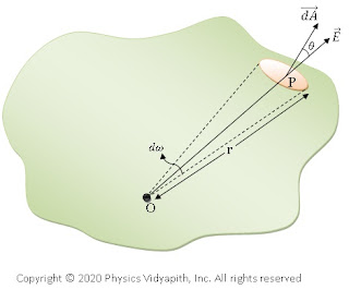 |
| When charge is inside the surface |

The total electric flux over the entire surface due to an external charge is zero.
- Electric field intensity due to a point charge
- Electric field intensity due to uniformly charged spherical Shell (for Thin and Thick)
- Electric field intensity due to a uniformly charged solid sphere (Conducting and Non-conducting)
- Electric field intensity due to uniformly charged infinite plane sheet (for Thin and Thick)
- Electric field intensity due to uniformly charged parallel sheet
- Electric field intensity due to charged infinite length wire
Popular Posts
-
 Derivation→ Let us consider, The charge on a parallel-plate capacitor = $q$ The area of parallel-plate = $A$ The dis...
 -
 Derivation→ Let us consider, a current-carrying conductor $XY$ having length $l$ in which current $i$ is flowing from $X$ to $Y$. Now,...
 -
 A.) Electric field intensity at different points in the field due to the uniformly charged solid conducting sphere: Let us consider, A s...
 -
 Description: The motion of any particle is depends upon the force applying on it. In the magnetic field, the motion of charge is perp...
 -
Principle of Ruby Laser → Ruby laser is the first working laser that was invented by T.H.Maima in 1960. It is a three-level solid-stat...
-
 Derivation of electric field intensity due to the uniformly charged wire of infinite length: Let us consider a uniformly-charged (positi...
 -
 Electric Potential due to an Electric Dipole: The electric potential due to an electric dipole can be measured at different points: ...
 -
Prove that: Group velocity is equal to Particle Velocity Solution: We know that group velocity $V_{g}=\frac{d\omega}{dk}$ $V_{g}=...
-
 Alternating Current Circuit Containing Inductance only (L-Circuit): Let us consider, An alternating current circuit containing a coil of i...
 -
Gauss's Law: Gauss's law for electric flux is given by Carl Friedrich Gauss in 1813. He extended the work of Joseph-Louis Lagr...

