Magnetic potential energy:
When a current carrying loop is placed in an external magnetic field the torque is acted upon the current loop which tends to rotate the current loop in a magnetic field. Therefore the work is done to change the orientation of the current loop against the torque. This work is stored in the form of magnetic potential energy in the current loop. This is known as the magnetic potential energy of the current loop.
Note: The current loop has magnetic potential energy depending upon its orientation in the magnetic field.
Derivation of Potential energy of current-loop in a magnetic field:
Let us consider, A current loop of magnetic moment $\overrightarrow{m}$ is held with its axis at an angle $\theta$ with the direction of a uniform magnetic field $\overrightarrow{B}$. The magnitude of the torque acting on the current loop or magnetic dipole is
$\tau=m \: B \: sin\theta \qquad(1)$
Now, the current loop is rotated through an infinitesimally small angle $d\theta$ against the torque. The work done to rotate the current loop
$dW=\tau \: d\theta$
$dW=m \: B \: sin\theta \: d\theta $ {from equation $(1)$}
If the current loop is rotated from an angle (or orientation) $\theta_{1}$ to $\theta_{2}$ then the work done
$W=\int_{\theta_{1}}^{\theta_{2}} m \: B \: sin\theta d\theta$
$W= m \: B \: \left[ -cos\theta \right]_{\theta_{1}}^{\theta_{2}} $
$W= m \: B \: \left( cos\theta_{1} - cos\theta_{2} \right) $
This work is stored in the form of potential energy $U$ of the current loop :
$U= m \: B \: \left( cos\theta_{1} - cos\theta_{2} \right) $
If $\theta_{1}=90^{\circ}$ and $\theta_{2}= \theta$
$U= m \: B \: \left( cos90^{\circ} - cos\theta \right) $
$U= - m \: B \: cos\theta $
$U= - \overrightarrow{m} . \overrightarrow{B}$
Thus, a current loop has minimum potential energy when $\overrightarrow{m}$ and $\overrightarrow{B}$ are parallel and maximum potential energy when $\overrightarrow{m}$ and $\overrightarrow{B}$ are antiparallel.
Magnetic Dipole Moment of Current carrying loop
Current carrying Loop or Coil or Solenoid:
The current carrying loop (or Coil or solenoid) behaves like a bar magnet. A bar magnet with the north and south poles at its ends is a magnetic dipole, so a current -loop is also a magnetic dipole.
Equation of Magnetic Dipole Moment of Current carrying Loop:
When a current loop is suspended in a magnetic field, it experiences the torque which tends to rotate the current loop to a position in which the axis of the loop is parallel to the field. So the magnitude of the torque acting on the current loop in the uniform magnetic field $\overrightarrow{B}$ is given by:
$\tau=iAB sin\theta \qquad(1)$
Where $A$ - Area of the current loop
We also know that when the electric dipole is placed in the electric field, it also experiences the torque which tends to rotate the electric dipole in the electric field. So the magnitude of the torque on the electric dipole in the uniform electric field $\overrightarrow{E}$ is given by:
$\tau=pE sin\theta \qquad(2)$
Where $p$ - The magnitude of the electric dipole moment
Now compare the equation $(1)$ and equation $(2)$ and we can conclude that the current loop also has a magnetic dipole moment just like an electric dipole have an electric dipole moment. The magnetic dipole moment is associated with the current in the loop and the area of the current loop. It is represented by $\overrightarrow {m}$. So the magnitude of the magnetic dipole moment of current carrying loop is:
$m=iA$
The vector form of the magnetic dipole moment current carrying loop is
$\overrightarrow{m} = i\overrightarrow{A}$
The magnetic dipole moment of current carrying coil:
If the current-carrying loop has $N$ number of turns (i.e current carrying coil) then the magnetic dipole moment of current carrying coil:
$m=NiA$
The vector form of the magnetic dipole moment of the current carrying coil is
$\overrightarrow{m} =N i\overrightarrow{A}$
The magnetic dipole moment of Circular Loop:
Let us consider the circular loop of radius $a$ in which current $i$ is flowing the magnitude of the magnetic dipole moment of the circular loop:
$m=i A$
Here the area $A$ of the circular loop is $\pi a^{2}$ then the magnitude of the magnetic dipole moment of the circular loop is:
$m=i \pi a^{2} \qquad(3)$
The magnetic field at the center of the current carrying a circular loop in terms of current is:
$B=\frac{\mu_{\circ}i}{2a}$
Now substitute the value of $i$ from equation $(3)$ in the above equation then the magnetic field at the center of the current carrying circular loop in terms of magnetic dipole moment is:
$B=\frac{\mu_{\circ}m}{2\pi a^{3}}$
$B=\frac{\mu_{\circ}}{4\pi} \frac{2m}{a^{3}}$
Force between two long and parallel current-carrying conductor
Derivation of Force between two long and parallel current-carrying conductors:
Let us consider:
The two long straight, parallel conductors = $PQ$ and $RS$
The length of the conductor= $l$
The distance between the parallel conductor = $r$
The current flowing in conductor $PQ$ = $i_{1}$
The current flowing in conductor $RS$ = $i_{2}$
The magnetic field due to conductor $PQ$ = $B_{1}$
The magnetic field due to conductor $RS$ = $B_{2}$
The magnetic force on conductor $PQ$= $F_{1}$
The magnetic force on conductor $RS$= $F_{2}$
Now Consider the magnetic force on conductor $RS$ is i.e.
$F_{2}=i_{2}B_{1}l sin\theta$
Where $\theta$ is the angle between the magnetic field and length element of conductor i.e. $\theta=90^{\circ}$ so above equation can be written as,
$F_{2}=i_{2}B_{1}l sin 90^{\circ}$
$F_{2}=i_{2}B_{1}l \qquad(1)$
The magnetic field due to conductor PQ is:
$B_{1}= \frac{\mu_{\circ}}{2\pi} \frac{i_{1}}{r}$
Now substitute the value of $B_{1}$ in equation $(1)$ so the force on conductor $RS$
$F_{2}=\frac{\mu_{\circ}}{2\pi} \frac{i_{1}i_{2}}{r}l $
So the force per unit length on the conductor $RS$ is
$\frac{F_{2}}{l}=\frac{\mu_{\circ}}{2\pi} \frac{i_{1}i_{2}}{r} \qquad(2)$
Similarly, we can solve the force per unit length on the conductor $PQ$
$\frac{F_{1}}{l}=\frac{\mu_{\circ}}{2\pi} \frac{i_{1}i_{2}}{r} \qquad(3)$
So from the above equation, we can conclude that the force per unit length is the same on both conductors whether both have different amounts of current flowing. The generalized form of the force per unit length from the above equations is
$\frac{F}{l}=\frac{\mu_{\circ}}{2\pi} \frac{i_{1}i_{2}}{r}$
Note: When both parallel conductors have the same direction of current then the force between the conductor will be repulsive. or when both parallel conductors have opposite directions of current then the force between the conductor is attractive.
 |
| Force Between Parallel Current Carrying Conductor |
Force on current carrying conductor in uniform magnetic field
Derivation of force on current-carrying conductor in uniform magnetic field:
Let us consider:
The length of the conductor - $l$
The cross-section area of the current carrying conductor - $A$
The current flow in a conductor- $i$
The drift or average velocity of the free electrons - $v_{d}$
The current-carrying conductor is placed in a magnetic field - $B$
The total number of free electrons in the current carrying conductor - $N$
Now the magnetic force on one free electron in a conductor -
$F'= ev_{d}B sin\theta \qquad(1)$
The net force on the conductor is due to all the free electrons present in the conductor
$F=N\: F' \qquad(2)$
Let $N$ is the number of free electrons per unit volume of conductor. So the total number of free electrons in the $Al$ volume of the conductor will be
$N=nAl \qquad(3)$
Now substitute the value of $N$ and $F'$ from above equation $(1)$ and equation $(3)$ in equation $(2)$
$F=neAlv_{d}B\: sin\theta$
Where $i=neAv_{d}$
So from the above equation
$F=ilB \: sin\theta $
The Vector Form of the above equation:
$F=i \left(\overrightarrow{l} \times \overrightarrow{B} \right) $
Let us consider, a conductor of length of $l$ in which $i$ current carrying is flowing and placed in magnetic field $B$ at an angle $\theta$. If $i$ current is flowing in the conductor then magnetic force on the conductor depends upon
1) The magnetic force is directly proportional current.
$F \propto i \qquad(1)$
2.) The magnetic force is directly proportional to the length of the conductor.
$F \propto l \qquad(2)$
3.) The magnetic force is directly proportional to the magnetic field.
$F \propto B \qquad(3)$
4.) The magnetic force is directly proportional to the $sin \theta$. Here $\theta$ is the angle between the length of the current element and the magnetic field.
$F \propto sin \theta \qquad(4)$
from equation $(1)$, $(2)$, $(3)$, and equation $(4)$
$F \propto i \: l \: B sin\theta$
$F = k \: i \: l \: B sin\theta$
Here $k$ is constant which has value $1$, then above equation
$F = i\: l \: b \: sin\theta$
Vector form of the above equation:
$F = i \left( \overrightarrow{l} \times \overrightarrow{B} \right)$
 |
| Force on current carrying conductor in the uniform magnetic field |
Alternative Method
Principle, Construction and Working of Current Carrying Solenoid
Current Carrying Solenoid:
The Solenoid is an artificial magnet which is used for different purposes.
Principle of Solenoid:
The principle of the solenoid is based on the "Ampere Circuital Law" and its magnetic field is raised due to the current carrying a circular loop.
Construction of Solenoid:
The current carrying solenoid is consist of insulated cylindrical material and conducting wire. The conducting wire like copper is wrapped closely around the insulated cylindrical material ( like cardboard, clay, or plastic). The end faces of the conducting wire are connected to the battery.
Working:
When the electric current flow in the solenoid then a field (i.e. Magnetic field) is produced around and within the current carrying solenoid. This magnetic field is produced in solenoid due to circular loops of the solenoid and the direction of the magnetic field is depend upon the direction of the electric current flow in the circular loop. The magnetic field within the current carrying solenoid is uniform and parallel to the axis of the solenoid.
Derivation of the magnetic field due to long current carrying Solenoid:
Let us consider a very long current carrying solenoid of length $l$ in which $i$ electric current is flowing. Here its diameter is very less as compared to the length of the solenoid.
Now take a closed rectangular path $abcd$ in which the side $ab$ is parallel to the axis of the solenoid and sides $bc$ and $da$ are very long so that the side $cd$ is far from the solenoid and the magnetic field at this side is negligibly small.
Now apply Ampere's circuital law to the rectangular path $abcd$
$\oint \overrightarrow{B}. \overrightarrow{dl}=\mu_{\circ} i' \qquad(1)$
Where $i'$ is the current enclosed by the rectangle.
Let $n$ is the number of turns per unit length of the solenoid. So the number of turns in a length $x$ is = $nx$
The current in each turn is $i$ then the net current $(i')$ enclosed by the rectangle $abcd$ is $nxi$ i.e
$i'=nxi$
Now substitute the value of $i'$ in above equation $(1)$
$\oint \overrightarrow{B}. \overrightarrow{dl}=\mu_{\circ} nxi \qquad(2)$
Now expand the Ampere circuital law for closed rectangular $abcd$-
In above equation the term:
$\int_{b}^{c} \overrightarrow{B}.\overrightarrow{dl}= \int_{d}^{a} \overrightarrow{B}.\overrightarrow{dl}=0$
The above term is zero because along $bc$ and $da$ the magnetic field $\overrightarrow{B}$ and length element $\overrightarrow{dl}$ are perpendicular to each other.
$\int_{c}^{d} \overrightarrow{B}.\overrightarrow{dl}=0 $
The above term is zero because the magnetic field $\overrightarrow{B}$ outside the solenoid is negligible due long length of the solenoid.
The above equation $(3)$ can be written by applying the above condition-
$\oint \overrightarrow{B}.\overrightarrow{dl}=\int_{a}^{b} \overrightarrow{B}.\overrightarrow{dl}$
$\oint \overrightarrow{B}.\overrightarrow{dl}= \overrightarrow{B}\int_{a}^{b} \overrightarrow{dl}$
$\oint \overrightarrow{B}.\overrightarrow{dl}= B x \qquad(4)$
Where $x$- Length of $ab$
From equation $(2)$ and equation $(4)$, we get
$Bx=\mu_{\circ}nxl$
$B=\mu_{\circ}nl$
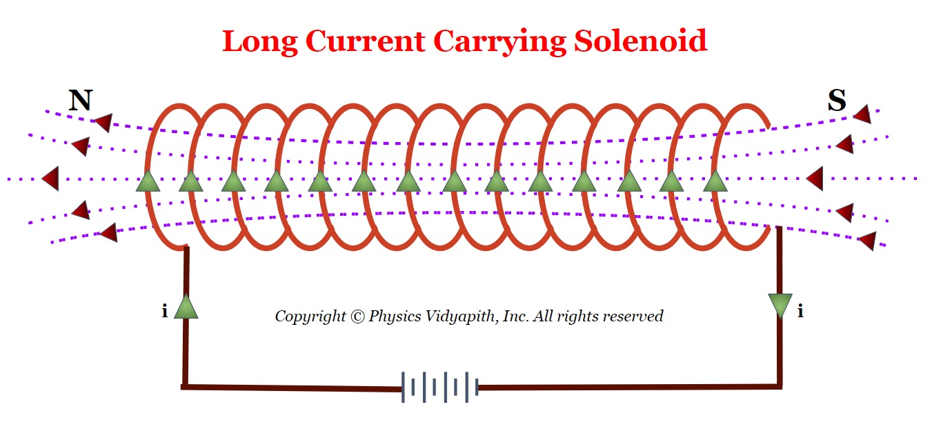 |
| Long Current Carrying Solenoid |
 |
| Cross Section View of the long Current Carrying Solenoid |
$\oint \overrightarrow{B}.\overrightarrow{dl}=\int_{a}^{b} \overrightarrow{B}.\overrightarrow{dl}+ \int_{b}^{c} \overrightarrow{B}.\overrightarrow{dl} + \int_{c}^{d} \overrightarrow{B}.\overrightarrow{dl} + \int_{d}^{a} \overrightarrow{B}.\overrightarrow{dl} \qquad(3)$
Comparison of Step Index and Graded Index Fibres
Comparison of Step Index Fibres and Graded Index Fibres(GRIN)→
| S.No. | Step Index Fibre | Graded Index Fibre |
|---|---|---|
| 1. | In a step-index fibre, the refractive index of the core a constant value. | In graded-index fibre, the refractive index in the core decreases continuously in a nearly parabolic manner from a maximum value at the centre of the core to a constant value at the core-cladding interface. |
| 2. |
For a step-index fibre, the variation of refractive index is mathematically expressed as,
$\begin{cases} & \mu(r)=\mu_{1} \qquad 0 < r < a \quad for (core)\\ & \mu(r)=\mu_{2} \qquad r >a \quad for(Cladding)\\ \end{cases} \\ Where \: \mu_{1} > \mu{2} $ |
Parabolic refractive index variation in GRIN fibre is mathematically expressed as,
$ \begin{cases} & \mu^{2}(r)=\mu^{2}_{1} \left[ 1- \left(\frac{r}{\alpha} \right)^{2} \right] \qquad 0 < r < a \quad for (core) \\ & \mu(r)=\mu^{2}_{2} \qquad \qquad \qquad \qquad r > a \quad for (Cladding) \end{cases} $ |
| 3. | In the step-index fibre, the propagating light rays reflect abruptly from the Core cladding boundary. | In graded-index fibre, the propagating light rays bend smoothly as they approach the cladding. |
| 4. | for given fibre diameter, the numerical aperture of step-index fibre is large. | For the same fibre diameter, the numerical aperture of graded-index fibre is small. |
| 5. | In the step-index fibre, there may be some irregularities at the interface between the core and cladding. | In the graded-index fibre, there are no such irregularities at the interface between core and cladding. |
| 6. | The step-index fibre has higher attenuation. | The graded-index fibre has lower attenuation. |
| 7. | For a step-index fibre of a given physical size, with a loss of power of the order of $12 \frac{dB}{km}$, the numerical aperture is of the order of $0.2$ to $0.35$. | For a graded-index fibre of the same physical size, with an attenuation between $5$ to $10 \frac{dB}{km}$, the numerical aperture tends to run between $0.16$ and $0.2$ |
| 8. |
In step index fibre, the time interval at the output end or pulse dispersion is expressed as,
$\Delta \tau = \frac{\mu_{1} l}{c} \left ( \frac{\mu_{1}}{\mu_{2}} - 1 \right)=\frac{\mu_{1} l}{c} \Delta$ Where $l$ → The length of the fibre. |
In a graded index fibre, the time interval at the output end or pulse dispersion is expressed as,
$\Delta \tau = \frac{\mu_{2} l}{2c} \left ( \frac{\mu_{1} - \mu_{2}} {\mu_{2}} \right)^{2}=\frac{\mu_{2} l}{2c} \Delta^{2}$ Where $l$ → The length of the fibre. |
| 9. | Pulse dispersion in multimode step-index fibre is large. | Pulse dispersion in a graded-index fibre is small. |
| 10. | A good quality step-index fibre may have a bandwidth of $50 MHz km$ | The equivalent graded-index fibre can have $200$, $400$, or $600 MHz km$ bandwidth. |