We have assumed that the wave associated with a particle in motion is represented by a complex variable quantity called the wave function $\psi(x,t)$. Therefore, it can not have a direct physical meaning. Since it is a complex quantity, it may be expressed as
$\psi(x,y,z,t)=a+ib \qquad(1)$
Where $a$ and $b$ are real functions of the variable $(x,y,z,t)$. The complex conjugate of wave function $\psi(x,y,z,t)$
$\psi^{*}(x,y,z,t)=a-ib \qquad(2)$
Multiply equation $(1)$ and equation $(2)$
$\psi(x,y,z,t).\psi^{*}(x,y,z,t)=a^{2}+b^{2} \qquad(3)$
$ \left| \psi(x,y,z,t) \right|^{2}=a^{2}+b^{2} \qquad(4)$
If $\psi \neq 0$ Then the product of $\psi$ and $\psi^{*}$ is real and positive. Its positive square root is denoted by $\left|\psi(x,y,z,t) \right|$, and it is called the modulus of $\psi$.
The quantity $ \left| \psi(x,y,z,t) \right|^{2}$ is called the probability density $(P)$. So for the motion of a particle, the probability of finding the particle in the region $d\tau$ will be:
$\int {P d\tau}= \int {\psi(x,y,z,t).\psi^{*}(x,y,z,t).d\tau}=\int {\left| \psi(x,y,z,t) \right|^{2}d\tau}$
Here $P$ are the probability that tells us that the particle will be found in a volume element $d\tau(=dx.dy.dz)$ surrounding the point at position $(x,y,z)$ at time $t$.
For the motion of a particle in one dimension, the probability of finding the particle in the region $dx$ will be:
$\int{P dx}= \int {\psi(x,t).\psi^{*}(x,t).dx}=\int {\left| \psi(x,t) \right|^{2}dx}$
Energy flow in the electromagnetic wave in free space
Derivation of energy flow in the electromagnetic wave in free space:
The Poynting vector is given by
$\overrightarrow{S}=\overrightarrow{E} \times \overrightarrow{H} \qquad(1)$
$\overrightarrow{S}=\frac{1}{\mu_{0}} ( \overrightarrow{E} \times \overrightarrow{B} ) \qquad(2) \qquad (\because \overrightarrow{B}= \mu_{0} \overrightarrow{H})$
We know that the characteristic impedance equation i.e.
$\overrightarrow{B}=\frac{1}{\mu_{0}c}(\hat{n} \times \overrightarrow{E}) \qquad(3)$
Now substitute the value of $\overrightarrow{B}$ in equation$(2)$
$\overrightarrow{S}=\frac{1}{\mu_{0}c} [\overrightarrow{E} \times (\hat{n} \times \overrightarrow{E})]$
$\overrightarrow{S}=\frac{1}{\mu_{0}c} [(\overrightarrow{E}.\overrightarrow{E}) \hat{n}- (\overrightarrow{E}.\hat{n}) \overrightarrow{E})] \qquad(4)$
As $\overrightarrow{E}$ is perpendicular to $\hat{n}$ so $\overrightarrow{E} . \hat{n}=0$ then we get for above equation$(4)$
$\overrightarrow{S}=\frac{1}{\mu_{0}c} E^{2} \hat{n}$
From the above equation, we can conclude $\overrightarrow{S}$ has the same direction as $\hat{n}$ which is the direction of wave propagation.
Energy flow in an electromagnetic wave takes place in the direction of the propagation of the wave.
Here $\mu_{0} c=Z_{0}$ (The Characteristic impedance of free space)
$\overrightarrow{S}=\frac{1}{Z_{0}} E^{2} \hat{n}$
This is the equation of energy flow in the electromagnetic wave in free space.
The average energy flow over one period of the electromagnetic wave in free space:
Now the average energy flow of the above equation
$ \left< \overrightarrow{S} \right> =\frac{1}{Z_{0}} \left< E^{2} \right> \hat{n} \qquad(5)$
We know the electric field vector wave equation i.e. $\overrightarrow{E}=E_{0} e^{i(\overrightarrow{k}. \overrightarrow{r} -\omega t)} $
So the value of $\left< E^{2} \right>$ from above equation:
$\left< E^{2} \right>= \left< Re[E_{0} e^{i(\overrightarrow{k}. \overrightarrow{r} -\omega t)}]^{2} \right>$
$\left< E^{2} \right>= \left< E_{0}^{2}\: cos^{2}(\overrightarrow{k}. \overrightarrow{r} -\omega t) \right>$
For one period or cycle of electromagnetic wave the value of $cos^{2}(\overrightarrow{k}. \overrightarrow{r} -\omega t)=\frac{1}{2}$ then we get
$\left< E^{2} \right>= \frac{E_{0}^{2}}{2}$
$\left< E^{2} \right>= (\frac{E_{0}}{2})^{2}$
$\left< E^{2} \right>= E_{rms}^{2} \qquad \left (\because E_{rms} = \frac{E_{0}}{2}\right )$
Now substitute the value of $ \left< E^{2} \right>$ in equation $(5)$ then we get
$ \left< \overrightarrow{S} \right> =\frac{E_{rms}^{2}}{Z_{0}} \hat{n} $
This average energy flow equation over one period of the electromagnetic wave in free space.
Momentum of electromagnetic wave
Derivation of momentum of electromagnetic wave:
Maxwell's had also predicted that electromagnetic waves transport linear momentum in the direction of propagation. Let a particle which has mass $m$ moving with velocity then the momentum of a particle,
$\overrightarrow{P}=m\overrightarrow{v} \qquad(1)$
According to mass-energy relation
$U=mc^{2}$
Here $U$ - Total energy of the particle
$m=\frac{U}{c^{2}} \qquad(2)$
From equation $(1)$ and equation $(2)$
$\overrightarrow{P}=\frac{U}{c^{2}} \overrightarrow{v} \qquad(3)$
If the electromagnetic wave is propagating along the x-axis then
$\overrightarrow{v}=c \hat{i}$
Put this value in the above equation $(3)$
$\overrightarrow{P}=\frac{U}{c} \hat{i} \qquad(4)$
We know that the equation of energy flow in electromagnetic wave
$\overrightarrow{S}= \frac{1}{\mu_{0} c} E^{2} \hat{n}$
Here wave is propagating along x-axis i.e
$\hat{n}=\hat{i}$
$\overrightarrow{S}= \frac{1}{\mu_{0} c} E^{2} \hat{i} \qquad(5)$
The energy density in plane electromagnetic wave in free space:
$U=\epsilon_{0} E^{2}$
Where $E$ - Magnitude of electric field
$E^{2}=\frac{U}{\epsilon_{0}} \qquad(6)$
Now substitute the value of $E^{2}$ in equation$(5)$
$\overrightarrow{S}= \frac{1}{\mu_{0} c} \frac{U}{\epsilon_{0}} \hat{i} $
$\overrightarrow{S}= \frac{c^{2}}{c} U \hat{i} \qquad (\because \frac{1}{\sqrt{ \mu_{0} \epsilon_{0}}}=c) $
$\overrightarrow{S}= c U \hat{i} $
$U \hat{i}=\frac{\overrightarrow{S}}{c} \qquad(7)$
Now substitute the value of $ U \hat{i} $ in equation $(4)$. Then
$\overrightarrow{P}=\frac{\overrightarrow{S}}{c}$
$\overrightarrow{P}=\frac{(\overrightarrow{E} \times \overrightarrow{B})}{ \mu_{0}c^{2}}$
$\overrightarrow{P}=\epsilon_{0}(\overrightarrow{E} \times \overrightarrow{B})$
This is the equation of "Momentum of electromagnetic wave"
Particle in one dimensional box (Infinite Potential Well)
Let us consider a particle of mass $m$ that is confined to one-dimensional region $0 \leq x \leq L$ or the particle is restricted to move along the $x$-axis between $x=0$ and $x=L$. Let the particle can move freely in either direction, between $x=0$ and $x=L$. The endpoints of the region behave as ideally reflecting barriers so that the particle can not leave the region. A potential energy function $V(x)$ for this situation is shown in the figure below.
The potential energy inside the one -dimensional box can be represented as
$\begin{Bmatrix}
V(x)=0 &for \: 0\leq x \leq L \\
V(x)=\infty & for \: 0> x > L \\
\end{Bmatrix}$
$\frac{d^{2} \psi(x)}{d x^{2}}+\frac{2m}{\hbar^{2}}(E-V)\psi(x)=0 \qquad(1)$
If the particle is free in a one-dimensional box, Schrodinger's wave equation can be written as:
$\frac{d^{2} \psi(x)}{d x^{2}}+\frac{2mE}{\hbar^{2}}\psi(x)=0$
$\frac{d^{2} \psi(x)}{d x^{2}}+\frac{8 \pi^{2} mE}{h^{2}}\psi(x)=0 \quad (\because \hbar=\frac{h}{2 \pi}) \quad(2)$
$\frac{d^{2} \psi(x)}{d x^{2}}+ k^{2}\psi(x)=0 \quad (\because k^{2}=\frac{8 \pi^{2} mE}{h^{2}}) \quad(3)$
The general solution of the above differential equation $(2)$
$\psi(x)= A sin(kx)+ B cos(kx) \qquad(4)$
The wave function $\psi(x)$ should be zero everywhere outside the box since the probability of finding the particle outside the box is zero. Similarly, the wave function $\psi(x)$ must also be zero at walls of the box because the probability density $[\psi(x)]^{2}$ must be continuous. Thus, the boundary conditions for this problem is that
(i) $\psi(x)=0$ For $x=0$
(ii) $\psi(x)=0$ For $x=L$
Now applying the boundary condition in equation$(4)$ i.e.
(i) At $x=0$ the wave function $\psi(0)=0$
Now we get
$\psi(0)= A sin(k.0)+ B cos(k.0)$
$A sin(k.0)+ B cos(k.0)=0 \qquad (\because \psi(0)= 0)$
$B=0$
Hence substitute the value of $B$ in equation$(4)$ ,
$\psi(L)= A sin(kx) \qquad(5)$
Now applying the second boundary condition:
(ii) At $x=L$ the wave function $\psi(L)=0$, we get
$\psi(x)= A sin(kL) \qquad(6)$
This equation will satisfy only for certain values of $k$, say $k_{n}$. Since $A$ can not be taken zero hence
$sin(k_{n}L)=0 $
$sin(k_{n}L)=sin(n\pi) $
$k_{n}L=n\pi $
$k_{n}=\frac{n\pi}{L} \qquad(7)$
Thus for each allowed values of $k_{n}$ there is a wave function $\psi(x)$ given as, using equation$(5)$ and equation$(7)$
$\psi_{n}(x)=A sin(\frac{n\pi x}{L})$
This is the expression of the wave function or eigen function for a particle in a box.
Now, from equation $(3)$ and equation$(7)$, we get
$k^{2}=\frac{8 \pi^{2} mE}{h^{2}}= (\frac{n \pi}{L})^{2}$
$E=\frac{n^{2} h^{2}}{8mL^{2}}$
This is the expression of energy or eigen value for a particle in a box.
In general, the expression for this energy is written as:
$E_{n}=\frac{n^{2} h^{2}}{8mL^{2}}$
For different values of $n$ energy values can be written as
For $n=1$
$E_{1}=\frac{h^{2}}{8mL^{2}}$
It is known as zero-point energy or ground energy state
For $n=2$
$E_{2}=\frac{2^{2} h^{2}}{8mL^{2}}=2^{2}E_{1}$
For $n=3$
$E_{3}=\frac{3^{2} h^{2}}{8mL^{2}}=3^{2}E_{1}$
For $n=4$
$E_{4}=\frac{4^{2} h^{2}}{8mL^{2}}=4^{2}E_{1}$
So generalized form of the above equation can be written as
$E_{n}=n^{2}E_{1}$
Some of the possible energies for a particle in a box are shown on an energy-level diagram in the figure below.
The energy levels have a spacing that increases with increasing $n$ and thus the particle in a box can take only certain discrete energy values, called Eigen-values. This means that the energy levels of a particle in a box are quantized but according to classical mechanics, the particle may take any continuous range of energy values between zero and infinity.
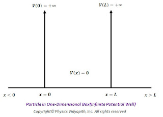 |
Particle in One-Dimensional Box(Infinite Potential Well) |
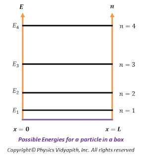 |
Possible Energies for a particle in a box |
Solution of electromagnetic wave equations in free space
The electromagnetic wave equations in free space:
For electric field vector:
$\nabla^{2} \overrightarrow{E}=\frac{1}{c^{2}} \frac{\partial^{2} \overrightarrow{E}}{\partial t^{2}} \qquad(1)$
For magnetic field vector:
$\nabla^{2} \overrightarrow{B}=\frac{1}{c^{2}} \frac{\partial^{2} \overrightarrow{B}}{\partial t^{2}} \qquad(2)$
The wave equation of electric field vector:
$\overrightarrow{E}(\overrightarrow{r},t)=E_{\circ} e^{i(\overrightarrow{k}. \overrightarrow{r} - \omega t)} \qquad(3)$
The wave equation of magnetic field vector:
$\overrightarrow{B}(\overrightarrow{r},t)=B_{\circ} e^{i(\overrightarrow{k}. \overrightarrow{r} - \omega t)} \qquad(4)$
Now the solution of electromagnetic wave for electric field vector.
Differentiate with respect to $t$ of equation $(3)$
$\frac{\partial \overrightarrow{E}}{\partial t}=i \omega E_{\circ} e^{i(\overrightarrow{k}. \overrightarrow{r} - \omega t)}$
Again differentiate with respect to $t$ of the above equation:
$\frac{\partial^{2} \overrightarrow{E}}{\partial t^{2}}=i^{2} \omega^{2} E_{\circ} e^{i(\overrightarrow{k}. \overrightarrow{r} - \omega t)}$
$\frac{\partial^{2} \overrightarrow{E}}{\partial^{2} t}=- \omega^{2} \overrightarrow{E}(\overrightarrow{r},t)$
Now substitute the value of the above equation in equation$(1)$
$\nabla^{2} \overrightarrow{E}=\frac{-\omega^{2}}{c^{2}} \overrightarrow{E}(\overrightarrow{r},t)$
$\nabla^{2} \overrightarrow{E}=-(\frac{\omega}{c})^{2} \overrightarrow{E}(\overrightarrow{r},t)$
$\nabla^{2} \overrightarrow{E}=-k^{2} \overrightarrow{E}(\overrightarrow{r},t) \qquad (\because \frac{\omega}{c}=k )$
Where $k$ - Wave propagation Constant
$\nabla^{2} \overrightarrow{E} + k^{2} \overrightarrow{E}(\overrightarrow{r},t)=0 $
This is the solution of the electromagnetic wave equation in free space for the electric field vector.
Now the component form of the above equation:
$(\frac{\partial^{2}}{\partial x^{2}}
+ \frac{\partial^{2}}{\partial y^{2}} +\frac{\partial^{2}}{\partial z^{2}})(\hat{i}E_{x}+\hat{j}E_{y}+\hat{k}E_{z}) \\ =- k^{2}(\hat{i}E_{x}+\hat{j}E_{y}+\hat{k}E_{z}) \qquad(5)$
If the wave is propagating along $z$ direction. Then for uniform-plane electromagnetic waves-
$\frac{\partial}{\partial x}=\frac{\partial}{\partial y}=0$
$\frac{\partial^{2}}{\partial x^{2}}=\frac{\partial^{2}}{\partial y^{2}}=0$
$E_{z}=0$
Now the equation $(5)$ can be written as:
$\frac{\partial^{2}}{\partial x^{2}}(\hat{i}E_{x}+\hat{j}E_{y})=- k^{2}(\hat{i}E_{x}+\hat{j}E_{y})$
Now separate the above equation in $x$ and $y$ components so
$\frac{\partial^{2} E_{x}}{\partial z^{2}}=- k^{2}E_{x}$
$\frac{\partial^{2}E_{y}}{\partial z^{2}} =- k^{2}E_{y}$
The solution of electromagnetic wave for magnetic field vector can find out by following the above method.
Therefore $x$ and $y$ components of the solution of the electromagnetic wave equation for magnetic field vector can be written as. i.e.
$\frac{\partial^{2} B_{x}}{\partial z^{2}}=- k^{2}B_{x}$
$\frac{\partial^{2}B_{y}}{\partial z^{2}} =- k^{2}B_{y}$
Derivation of time independent Schrodinger wave equation
Time independent Schrodinger wave equation:
We know the time dependent Schrodinger wave equation:
$i \hbar \frac{\partial \psi(x,t)}{\partial t}= -\frac{\hbar^{2}}{2m} \frac{\partial^{2} \psi(x,t)}{\partial x^{2}}+ V(x) \psi(x,t) \qquad(1)$
The wave function $\psi(x,t)$ is the product of space function $\psi(x)$ and time function $\psi(t)$. So
$\psi(x,t)=\psi(x) \psi(t) \qquad (2)$
Now apply the wave function form of equation$(2)$ to time dependent Schrodinger wave equation $(1)$
$i \hbar \psi(x) \frac{d \psi(t)}{d t}= -\frac{\hbar^{2}}{2m} \psi(t) \frac{d^{2} \psi(x)}{d x^{2}}+ V(x) \psi(x) \psi(t) \qquad(3)$
In the above equation $(3)$ ordinary derivatives is used in place of partial derivatives because each of function $\psi(x)$ and $\psi(t)$ depends on only one variable.
Now divide the above equation $(3)$ by $\psi(x)\psi(t)$ so
$i \hbar \frac{1}{\psi(t)} \frac{d \psi(t)}{d t}= -\frac{\hbar^{2}}{2m} \frac{1}{\psi(x)} \frac{d^{2} \psi(x)}{d x^{2}}+ V(x) \qquad(4)$
The above equation is known as the separation of time-independent part and time-independent part of the wave equation. The time-independent part is known as the energy function operator. i.e
$E=i \hbar \frac{1}{\psi(t)} \frac{d \psi(t)}{d t} \qquad(5)$
So from equation $(4)$ and equation$(5)$
$E= -\frac{\hbar^{2}}{2m} \frac{1}{\psi(x)} \frac{d^{2} \psi(x)}{d x^{2}}+ V(x)$
$E \psi(x)= -\frac{\hbar^{2}}{2m} \frac{d^{2} \psi(x)}{d x^{2}}+ V(x) \psi(x)$
$\frac{d^{2} \psi(x)}{d x^{2}}+\frac{2m}{\hbar^{2}}(E-V)\psi(x)=0$
This is time-independent Schrodinger wave equation.
Now for a free particle i.e, there is no force acting on the particle then the potential energy of a particle will be zero i.e. $V(x)=0$. Therefore time independent Schrodinger equation can be written as:
$\frac{d^{2} \psi(x)}{d x^{2}}+\frac{2mE}{\hbar^{2}}\psi(x)=0$
This is time-independent Schrodinger wave equation for a free particle.
Popular Posts
-
 Derivation→ Let us consider, The charge on a parallel-plate capacitor = $q$ The area of parallel-plate = $A$ The dis...
 -
 Derivation→ Let us consider, a current-carrying conductor $XY$ having length $l$ in which current $i$ is flowing from $X$ to $Y$. Now,...
 -
 A.) Electric field intensity at different points in the field due to the uniformly charged solid conducting sphere: Let us consider, A s...
 -
 Description: The motion of any particle is depends upon the force applying on it. In the magnetic field, the motion of charge is perp...
 -
Principle of Ruby Laser → Ruby laser is the first working laser that was invented by T.H.Maima in 1960. It is a three-level solid-stat...
-
 Derivation of electric field intensity due to the uniformly charged wire of infinite length: Let us consider a uniformly-charged (positi...
 -
Gauss's Law: Gauss's law for electric flux is given by Carl Friedrich Gauss in 1813. He extended the work of Joseph-Louis Lagr...
-
 Electric Potential due to an Electric Dipole: The electric potential due to an electric dipole can be measured at different points: ...
 -
Prove that: Group velocity is equal to Particle Velocity Solution: We know that group velocity $V_{g}=\frac{d\omega}{dk}$ $V_{g}=...
-
 Alternating Current Circuit Containing Inductance only (L-Circuit): Let us consider, An alternating current circuit containing a coil of i...

