Particle in one dimensional box (Infinite Potential Well)

Let us consider a particle of mass $m$ that is confined to one-dimensional region $0 \leq x \leq L$ or the particle is restricted to move along the $x$-axis between $x=0$ and $x=L$. Let the particle can move freely in either direction, between $x=0$ and $x=L$. The endpoints of the region behave as ideally reflecting barriers so that the particle can not leave the region. A potential energy function $V(x)$ for this situation is shown in the figure below.

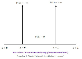
Particle in One-Dimensional Box(Infinite Potential Well)

The potential energy inside the one -dimensional box can be represented as

$\begin{Bmatrix} V(x)=0 &for \: 0\leq x \leq L \\ V(x)=\infty & for \: 0> x > L \\ \end{Bmatrix}$

$\frac{d^{2} \psi(x)}{d x^{2}}+\frac{2m}{\hbar^{2}}(E-V)\psi(x)=0 \qquad(1)$

If the particle is free in a one-dimensional box, Schrodinger's wave equation can be written as:

$\frac{d^{2} \psi(x)}{d x^{2}}+\frac{2mE}{\hbar^{2}}\psi(x)=0$

$\frac{d^{2} \psi(x)}{d x^{2}}+\frac{8 \pi^{2} mE}{h^{2}}\psi(x)=0 \quad (\because \hbar=\frac{h}{2 \pi}) \quad(2)$

$\frac{d^{2} \psi(x)}{d x^{2}}+ k^{2}\psi(x)=0 \quad (\because k^{2}=\frac{8 \pi^{2} mE}{h^{2}}) \quad(3)$

The general solution of the above differential equation $(2)$

$\psi(x)= A sin(kx)+ B cos(kx) \qquad(4)$

The wave function $\psi(x)$ should be zero everywhere outside the box since the probability of finding the particle outside the box is zero. Similarly, the wave function $\psi(x)$ must also be zero at walls of the box because the probability density $[\psi(x)]^{2}$ must be continuous. Thus, the boundary conditions for this problem is that

(i) $\psi(x)=0$ For $x=0$

(ii) $\psi(x)=0$ For $x=L$

Now applying the boundary condition in equation$(4)$ i.e.

(i) At $x=0$ the wave function $\psi(0)=0$

Now we get

$\psi(0)= A sin(k.0)+ B cos(k.0)$

$A sin(k.0)+ B cos(k.0)=0 \qquad (\because \psi(0)= 0)$

$B=0$

Hence substitute the value of $B$ in equation$(4)$ ,

$\psi(L)= A sin(kx) \qquad(5)$

Now applying the second boundary condition:

(ii) At $x=L$ the wave function $\psi(L)=0$, we get

$\psi(x)= A sin(kL) \qquad(6)$

This equation will satisfy only for certain values of $k$, say $k_{n}$. Since $A$ can not be taken zero hence

$sin(k_{n}L)=0 $

$sin(k_{n}L)=sin(n\pi) $

$k_{n}L=n\pi $

$k_{n}=\frac{n\pi}{L} \qquad(7)$

Thus for each allowed values of $k_{n}$ there is a wave function $\psi(x)$ given as, using equation$(5)$ and equation$(7)$

$\psi_{n}(x)=A sin(\frac{n\pi x}{L})$

This is the expression of the wave function or eigen function for a particle in a box.

Now, from equation $(3)$ and equation$(7)$, we get

$k^{2}=\frac{8 \pi^{2} mE}{h^{2}}= (\frac{n \pi}{L})^{2}$

$E=\frac{n^{2} h^{2}}{8mL^{2}}$

This is the expression of energy or eigen value for a particle in a box.

In general, the expression for this energy is written as:

$E_{n}=\frac{n^{2} h^{2}}{8mL^{2}}$

For different values of $n$ energy values can be written as

For $n=1$

$E_{1}=\frac{h^{2}}{8mL^{2}}$

It is known as zero-point energy or ground energy state

For $n=2$

$E_{2}=\frac{2^{2} h^{2}}{8mL^{2}}=2^{2}E_{1}$

For $n=3$

$E_{3}=\frac{3^{2} h^{2}}{8mL^{2}}=3^{2}E_{1}$

For $n=4$

$E_{4}=\frac{4^{2} h^{2}}{8mL^{2}}=4^{2}E_{1}$

So generalized form of the above equation can be written as

$E_{n}=n^{2}E_{1}$

Some of the possible energies for a particle in a box are shown on an energy-level diagram in the figure below.

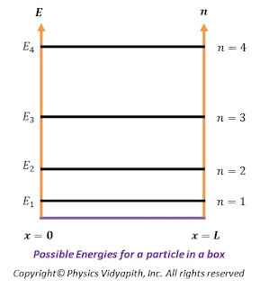
Possible Energies for a particle in a box

The energy levels have a spacing that increases with increasing $n$ and thus the particle in a box can take only certain discrete energy values, called Eigen-values. This means that the energy levels of a particle in a box are quantized but according to classical mechanics, the particle may take any continuous range of energy values between zero and infinity.

Read More

Solution of electromagnetic wave equations in free space

The electromagnetic wave equations in free space:

For electric field vector:

$\nabla^{2} \overrightarrow{E}=\frac{1}{c^{2}} \frac{\partial^{2} \overrightarrow{E}}{\partial t^{2}} \qquad(1)$

For magnetic field vector:

$\nabla^{2} \overrightarrow{B}=\frac{1}{c^{2}} \frac{\partial^{2} \overrightarrow{B}}{\partial t^{2}} \qquad(2)$

The wave equation of electric field vector:

$\overrightarrow{E}(\overrightarrow{r},t)=E_{\circ} e^{i(\overrightarrow{k}. \overrightarrow{r} - \omega t)} \qquad(3)$

The wave equation of magnetic field vector:

$\overrightarrow{B}(\overrightarrow{r},t)=B_{\circ} e^{i(\overrightarrow{k}. \overrightarrow{r} - \omega t)} \qquad(4)$

Now the solution of electromagnetic wave for electric field vector.

Differentiate with respect to $t$ of equation $(3)$

$\frac{\partial \overrightarrow{E}}{\partial t}=i \omega E_{\circ} e^{i(\overrightarrow{k}. \overrightarrow{r} - \omega t)}$

Again differentiate with respect to $t$ of the above equation:

$\frac{\partial^{2} \overrightarrow{E}}{\partial t^{2}}=i^{2} \omega^{2} E_{\circ} e^{i(\overrightarrow{k}. \overrightarrow{r} - \omega t)}$

$\frac{\partial^{2} \overrightarrow{E}}{\partial^{2} t}=- \omega^{2} \overrightarrow{E}(\overrightarrow{r},t)$

Now substitute the value of the above equation in equation$(1)$

$\nabla^{2} \overrightarrow{E}=\frac{-\omega^{2}}{c^{2}} \overrightarrow{E}(\overrightarrow{r},t)$

$\nabla^{2} \overrightarrow{E}=-(\frac{\omega}{c})^{2} \overrightarrow{E}(\overrightarrow{r},t)$

$\nabla^{2} \overrightarrow{E}=-k^{2} \overrightarrow{E}(\overrightarrow{r},t) \qquad (\because \frac{\omega}{c}=k )$

Where $k$ - Wave propagation Constant

$\nabla^{2} \overrightarrow{E} + k^{2} \overrightarrow{E}(\overrightarrow{r},t)=0 $

This is the solution of the electromagnetic wave equation in free space for the electric field vector.

Now the component form of the above equation:

$(\frac{\partial^{2}}{\partial x^{2}} + \frac{\partial^{2}}{\partial y^{2}} +\frac{\partial^{2}}{\partial z^{2}})(\hat{i}E_{x}+\hat{j}E_{y}+\hat{k}E_{z}) \\ =- k^{2}(\hat{i}E_{x}+\hat{j}E_{y}+\hat{k}E_{z}) \qquad(5)$

If the wave is propagating along $z$ direction. Then for uniform-plane electromagnetic waves-

$\frac{\partial}{\partial x}=\frac{\partial}{\partial y}=0$

$\frac{\partial^{2}}{\partial x^{2}}=\frac{\partial^{2}}{\partial y^{2}}=0$

$E_{z}=0$

Now the equation $(5)$ can be written as:

$\frac{\partial^{2}}{\partial x^{2}}(\hat{i}E_{x}+\hat{j}E_{y})=- k^{2}(\hat{i}E_{x}+\hat{j}E_{y})$

Now separate the above equation in $x$ and $y$ components so

$\frac{\partial^{2} E_{x}}{\partial z^{2}}=- k^{2}E_{x}$

$\frac{\partial^{2}E_{y}}{\partial z^{2}} =- k^{2}E_{y}$

The solution of electromagnetic wave for magnetic field vector can find out by following the above method.

Therefore $x$ and $y$ components of the solution of the electromagnetic wave equation for magnetic field vector can be written as. i.e.

$\frac{\partial^{2} B_{x}}{\partial z^{2}}=- k^{2}B_{x}$

$\frac{\partial^{2}B_{y}}{\partial z^{2}} =- k^{2}B_{y}$

Read More

Derivation of time independent Schrodinger wave equation

Time independent Schrodinger wave equation:

We know the time dependent Schrodinger wave equation:

$i \hbar \frac{\partial \psi(x,t)}{\partial t}= -\frac{\hbar^{2}}{2m} \frac{\partial^{2} \psi(x,t)}{\partial x^{2}}+ V(x) \psi(x,t) \qquad(1)$

The wave function $\psi(x,t)$ is the product of space function $\psi(x)$ and time function $\psi(t)$. So

$\psi(x,t)=\psi(x) \psi(t) \qquad (2)$

Now apply the wave function form of equation$(2)$ to time dependent Schrodinger wave equation $(1)$

$i \hbar \psi(x) \frac{d \psi(t)}{d t}= -\frac{\hbar^{2}}{2m} \psi(t) \frac{d^{2} \psi(x)}{d x^{2}}+ V(x) \psi(x) \psi(t) \qquad(3)$

In the above equation $(3)$ ordinary derivatives is used in place of partial derivatives because each of function $\psi(x)$ and $\psi(t)$ depends on only one variable.

Now divide the above equation $(3)$ by $\psi(x)\psi(t)$ so

$i \hbar \frac{1}{\psi(t)} \frac{d \psi(t)}{d t}= -\frac{\hbar^{2}}{2m} \frac{1}{\psi(x)} \frac{d^{2} \psi(x)}{d x^{2}}+ V(x) \qquad(4)$

The above equation is known as the separation of time-independent part and time-independent part of the wave equation. The time-independent part is known as the energy function operator. i.e

$E=i \hbar \frac{1}{\psi(t)} \frac{d \psi(t)}{d t} \qquad(5)$

So from equation $(4)$ and equation$(5)$

$E= -\frac{\hbar^{2}}{2m} \frac{1}{\psi(x)} \frac{d^{2} \psi(x)}{d x^{2}}+ V(x)$

$E \psi(x)= -\frac{\hbar^{2}}{2m} \frac{d^{2} \psi(x)}{d x^{2}}+ V(x) \psi(x)$

$\frac{d^{2} \psi(x)}{d x^{2}}+\frac{2m}{\hbar^{2}}(E-V)\psi(x)=0$

This is time-independent Schrodinger wave equation.

Now for a free particle i.e, there is no force acting on the particle then the potential energy of a particle will be zero i.e. $V(x)=0$. Therefore time independent Schrodinger equation can be written as:

$\frac{d^{2} \psi(x)}{d x^{2}}+\frac{2mE}{\hbar^{2}}\psi(x)=0$

This is time-independent Schrodinger wave equation for a free particle.

Read More

Derivation of time dependent Schrodinger's wave equation

Time-dependent Schrodinger wave equation:

Let a particle of mass $m$ is moving along the positive $x$-direction. So the total energy $E$ of the particle is:

$E=\frac{1}{2}mv^{2}+V(x)$

$E=\frac{(mv)^{2}}{2m}+V(x)$

$E=\frac{(P_{x}^{2})^{2}}{2m}+V(x) \qquad(1)$

Since moving particles are associated with the wave function $\psi(x,t)$. So multiply $\psi(x,t)$ on both sides of equation$(1)$

$E\psi(x,t) =\frac{(P_{x}^{2})^{2}}{2m} \psi(x,t)+V(x) \psi(x,t) \qquad(2)$

The wave function $\psi(x,t)$ representing the plane wave associated with the particle is given by:

$\psi(x,t)=A e^{\frac{i}{\hbar}(P_{x}.x-Et)} \qquad(3)$

Differentiate with respect to $x$ the above equation $(3)$

$\frac{\partial \psi(x,t)}{\partial x}= A e^{\frac{i}{\hbar}(P_{x}.x-Et)} (\frac{i}{\hbar})P_{x} \qquad(4)$

Again differentiate the above equation$(4)$

$\frac{\partial^{2} \psi(x,t)}{\partial x^{2}}= A e^{\frac{i}{\hbar}(P_{x}.x-Et)} (\frac{i}{\hbar})^{2}P_{x}^{2}$

$\frac{\partial^{2} \psi(x,t)}{\partial x^{2}}= - \frac{P_{x}^{2}}{\hbar ^{2}} \psi(x,t)$

$P_{x}^{2}\psi(x,t) =- \hbar^{2} \frac{\partial^{2} \psi(x,t)}{\partial x^{2}} \qquad(5)$

Now differentiate the equation $(3)$ with respect to $t$

$\frac{\partial \psi(x,t)}{\partial t}= A e^{\frac{i}{\hbar}(P_{x}.x-Et)} (\frac{i}{\hbar})(-E)$

$\frac{\partial \psi(x,t)}{\partial t}= - (\frac{i}{\hbar})E\psi(x,t)$

$\frac{\partial \psi(x,t)}{\partial t}= - (\frac{i}{\hbar})E\psi(x,t)$

$ E\psi(x,t)= -(\frac{\hbar}{i}) \frac{\partial \psi(x,t)}{\partial t}$

$ E\psi(x,t)= i^{2}(\frac{\hbar}{i}) \frac{\partial \psi(x,t)}{\partial t} \qquad (\because i^{2}=-1)$

$ E\psi(x,t)= i \hbar \frac{\partial \psi(x,t)}{\partial t} \qquad(6)$

Now substitute the value $E\psi(x,t)$ and $P_{x}^{2} \psi(x,t)$ in equation $(2)$. Then

$i \hbar \frac{\partial \psi(x,t)}{\partial t}= -\frac{\hbar^{2}}{2m} \frac{\partial^{2} \psi(x,t)}{\partial x^{2}}+ V(x) \psi(x,t)$

Thus above equation is time-dependent Schrodinger equation. Another form of the above equation can be written as:

$(i \hbar \frac{\partial}{\partial t}) \psi(x,t)= [-\frac{\hbar^{2}}{2m} \frac{\partial^{2}}{\partial x^{2}}+ V(x) ] \psi(x,t)$

Where
$i \hbar \frac{\partial}{\partial t}$→ Energy operator (E)

$-\frac{\hbar^{2}}{2m} \frac{\partial^{2}}{\partial x^{2}}+ V(x)$→ Hamiltonian operator(H)

Now above equation:

$E \psi(x,t)=H \psi(x,t)$

Read More

Solution of electromagnetic wave equations in non conducting media

The electromagnetic wave equations in non-conducting media :

For electric field vector:

$\nabla^{2} \overrightarrow{E}=\frac{1}{v^{2}} \frac{\partial^{2} \overrightarrow{E}}{\partial t^{2}} \qquad(1)$

For magnetic field vector:

$\nabla^{2} \overrightarrow{B}=\frac{1}{v^{2}} \frac{\partial^{2} \overrightarrow{B}}{\partial t^{2}} \qquad(2)$

The wave equation of electric field vector:

$\overrightarrow{E}(\overrightarrow{r},t)=E_{\circ} e^{i(\overrightarrow{k}. \overrightarrow{r} - \omega t)} \qquad(3)$

The wave equation of magnetic field vector:

$\overrightarrow{B}(\overrightarrow{r},t)=B_{\circ} e^{i(\overrightarrow{k}. \overrightarrow{r} - \omega t)} \qquad(4)$

Now the solution of electromagnetic wave for electric field vector.

Differentiate with respect to $t$ of equation $(3)$

$\frac{\partial \overrightarrow{E}}{\partial t}=i \omega E_{\circ} e^{i(\overrightarrow{k}. \overrightarrow{r} - \omega t)}$

Again differentiate with respect to $t$ of above equation:

$\frac{\partial^{2} \overrightarrow{E}}{\partial t^{2}}=i^{2} \omega^{2} E_{\circ} e^{i(\overrightarrow{k}. \overrightarrow{r} - \omega t)}$

$\frac{\partial^{2} \overrightarrow{E}}{\partial^{2} t}=- \omega^{2} \overrightarrow{E}(\overrightarrow{r},t)$

Now substitute the value of the above equation in equation$(1)$

$\nabla^{2} \overrightarrow{E}=\frac{-\omega^{2}}{v^{2}} \overrightarrow{E}(\overrightarrow{r},t)$

$\nabla^{2} \overrightarrow{E}=-(\frac{\omega}{v})^{2} \overrightarrow{E}(\overrightarrow{r},t)$

$\nabla^{2} \overrightarrow{E}=-\alpha^{2} \overrightarrow{E}(\overrightarrow{r},t) \qquad (\because \alpha=\frac{\omega}{v} )$

Where $\alpha$ - Wave propagation Constant

$\nabla^{2} \overrightarrow{E} + \alpha^{2} \overrightarrow{E}(\overrightarrow{r},t)=0 $

This is the solution of the electromagnetic wave equation in non-conducting media for the electric field vector.

Now the component form of the above equation:

$(\frac{\partial^{2}}{\partial x^{2}} + \frac{\partial^{2}}{\partial y^{2}} +\frac{\partial^{2}}{\partial z^{2}})(\hat{i}E_{x}+\hat{j}E_{y}+\hat{k}E_{z}) \\ =- \alpha^{2}(\hat{i}E_{x}+\hat{j}E_{y}+\hat{k}E_{z}) \qquad(5)$

If the wave is propagating along $z$ direction. Then for uniform-plane electromagnetic waves-

$\frac{\partial}{\partial x}=\frac{\partial}{\partial y}=0$

$\frac{\partial^{2}}{\partial x^{2}}=\frac{\partial^{2}}{\partial y^{2}}=0$

$E_{z}=0$

Now the equation $(5)$ can be written as:

$\frac{\partial^{2}}{\partial x^{2}} (\hat{i}E_{x}+\hat{j}E_{y})=- \alpha^{2}(\hat{i}E_{x}+\hat{j}E_{y})$

Now separate the above equation in $x$ and $y$ components so

$\frac{\partial^{2} E_{x}}{\partial z^{2}}=- \alpha^{2}E_{x}$

$\frac{\partial^{2}E_{y}}{\partial z^{2}} =- \alpha^{2}E_{y}$

The solution of electromagnetic wave for magnetic field vector can find out by following the above method.

Therefore $x$ and $y$ components of the solution of the electromagnetic wave equation for magnetic field vector can be written as. i.e.

$\frac{\partial^{2} B_{x}}{\partial z^{2}}=- \beta^{2}B_{x} \qquad \left( \because \beta=\frac{\omega}{v} \right)$

$\frac{\partial^{2}B_{y}}{\partial z^{2}} =- \beta^{2}B_{y}$

Read More

Difference between stable and unstable resonators

Difference between Stable and Unstable Resonators:

1. The oscillating beam is converged in stable resonator while in unstable resonator is spreads out of the the resonator.


2. In stable resonator laser output is from the centre of optical axis while in unstable resonator laser output comes from the edge of the output mirror.


3. The field is confined to the axis in stable resonator while it is not so in unstable resonator.


4. Stable resonators are used for low power lasers while unstable resonators are used for high power lasers.


5. In stable resonator these remains risk of breakage of the m  irrors while it is reduced to unstable resonators.


6. The mode volume is is small in stable resonators while it is large in unstable resonators.


7. The geometrical losses are large in unstable resonator in comparison to stable resonators.


8. In unstable resonators better beam quality may be achieved in comparison to stable resonators.

Read More